University of Windsor University of Windsor
Scholarship at UWindsor
Scholarship at UWindsor
Electronic Theses and Dissertations Theses, Dissertations, and Major Papers
1-1-2019
Digital Filter Design Using Improved Artificial Bee Colony
Digital Filter Design Using Improved Artificial Bee Colony
Algorithms
Algorithms
Rija RajuUniversity of Windsor
Follow this and additional works at: https://scholar.uwindsor.ca/etd
Recommended Citation Recommended Citation
Raju, Rija, "Digital Filter Design Using Improved Artificial Bee Colony Algorithms" (2019). Electronic Theses and Dissertations. 8177.
https://scholar.uwindsor.ca/etd/8177
This online database contains the full-text of PhD dissertations and Masters’ theses of University of Windsor students from 1954 forward. These documents are made available for personal study and research purposes only, in accordance with the Canadian Copyright Act and the Creative Commons license—CC BY-NC-ND (Attribution, Non-Commercial, No Derivative Works). Under this license, works must always be attributed to the copyright holder (original author), cannot be used for any commercial purposes, and may not be altered. Any other use would require the permission of the copyright holder. Students may inquire about withdrawing their dissertation and/or thesis from this database. For additional inquiries, please contact the repository administrator via email
Digital Filter Design Using Improved Artificial Bee Colony Algorithms
By
Rija Raju
A Dissertation
Submitted to the Faculty of Graduate Studies
through the Department of Electrical and Computer Engineering in Partial Fulfillment of the Requirements for
the Degree of Doctor of Philosophy at the University of Windsor
Windsor, Ontario, Canada
2019
Digital Filter Design Using Improved Artificial Bee Colony Algorithms
by
Rija Raju
APPROVED BY:
______________________________________________ W.-K. Ling, External Examiner
Guangdong University of Technology
______________________________________________ Z. Kobti
School of Computer Science
______________________________________________ H. Wu
Department of Electrical and Computer Engineering
______________________________________________ N. Kar
Department of Electrical and Computer Engineering
______________________________________________ H. K. Kwan, Advisor
Department of Electrical and Computer Engineering
iii
DECLARATION OF CO-AUTHORSHIP/ PREVIOUS PUBLICATION
I. Co-Authorship
I hereby declare that this dissertation incorporates material that is result of joint research, as follows:
This dissertation also incorporates the outcome of a joint research undertaken under the supervision of and in collaboration with my advisor Dr. H. K. Kwan. The collaborative work is covered mainly in Chapter 3, Chapter 4, Chapter 5 and Chapter 6 of the dissertation. In the dissertation, the contribution of ideas, the experimental designs, the data analysis and interpretation, and the writing were performed by the author, and the contribution of my advisor include the provision of ideas, the formulation of design problems, the analysis of the design results, and the writing and editing help. Dr. A. Jiang provided the MATLAB codes for the partial l1 optimization in [33] and programming advice.
I am aware of the University of Windsor Senate Policy on Authorship and I certify that I have properly acknowledged the contribution of other researchers to my dissertation and have obtained written permission from each of the co-author(s) to include the above material(s) in my dissertation.
I certify that, with the above qualification, this dissertation, and the research to which it refers, is the product of my own work.
II. Previous Publication
iv Dissertation
chapter
Publication title/full citation Publication
status
Chapter 3 H. K. Kwan and R. Raju, “Minimax design of linear phase FIR differentiators using artificial bee colony algorithm,” in Proc. of 8th International Conference on Wireless Communications and Signal Processing (WCSP 2016), Yangzhou, China, Oct. 13-15, 2016, pp. 1-4.
Published
Chapter 4 R. Raju, H. K. Kwan and A. Jiang, “Sparse FIR filter design using artificial bee colony algorithm,” in Proc. of IEEE 61st International Midwest Symposium on Circuits and Systems (MWSCAS 2018), Windsor, Ontario, Canada, Aug. 2018, pp. 956-959.
Published
Chapter 5 R. Raju and H. K. Kwan, “FIR filter design using multiobjective artificial bee colony algorithm,” in Proc. of 2017 IEEE 30th Canadian Conference on Electrical and Computer Engineering (CCECE 2017), Windsor, Ontario, Canada, Apr. 30-May 3, 2017, pp. 1-4.
Published
Chapter 6 R. Raju and H. K. Kwan, “IIR filter design using multiobjective artificial bee colony algorithm,” in Proc. of 2018 IEEE 31th Canadian Conference on Electrical and Computer Engineering (CCECE 2018), Quebec City, Quebec, Ontario, Canada, May 13-16, 2018, pp. 1-4.
v I certify that I have obtained a written permission from the copyright owners to include the above published materials in my dissertation. I certify that the above material describes work completed during my registration as graduate student at the University of Windsor.
I declare that, to the best of my knowledge, my dissertation does not infringe upon anyone’s copyright nor violate any proprietary rights and that any ideas, techniques, quotations, or any other material from the work of other people included in my dissertation, published or otherwise, are fully acknowledged in accordance with the standard referencing practices. Furthermore, to the extent that I have included copyrighted material that surpasses the bounds of fair dealing within the meaning of the Canada Copyright Act, I certify that I have obtained a written permission from the copyright owner(s) to include such material(s) in my dissertation and have included copies of such copyright clearances to my appendix.
vi
ABSTRACT
Digital filters are often used in digital signal processing applications. The design objective
of a digital filter is to find the optimal set of filter coefficients, which satisfies the desired
specifications of magnitude and group delay responses. Evolutionary algorithms are
population-based metaheuristic algorithms inspired by the biological behaviors of species.
Compared to gradient-based optimization algorithms such as steepest descent and
Newton’s like methods, these bio-inspired algorithms have the advantages of not getting
stuck at local optima and being independent of the starting point in the solution space. The
limitations of evolutionary algorithms include the presence of control parameters, problem
specific tuning procedure, premature convergence and slower convergence rate. The
artificial bee colony (ABC) algorithm is a swarm-based search metaheuristic algorithm
inspired by the foraging behaviors of honey bee colonies, with the benefit of a relatively
fewer control parameters. In its original form, the ABC algorithm has certain limitations
such as low convergence rate, and insufficient balance between exploration and
exploitation in the search equations. In this dissertation, an ABC-AMR algorithm is
proposed by incorporating an adaptive modification rate (AMR) into the original ABC
algorithm to increase convergence rate by adjusting the balance between exploration and
exploitation in the search equations through an adaptive determination of the number of
parameters to be updated in every iteration. A constrained ABC-AMR algorithm is also
developed for solving constrained optimization problems.
There are many real-world problems requiring simultaneous optimizations of more than
vii solutions called the Pareto front instead of a single optimum solution. For multiobjective
optimization, if a decision maker’s preferences can be incorporated during the optimization
process, the search process can be confined to the region of interest instead of searching
the entire region. In this dissertation, two algorithms are developed for such incorporation.
The first one is a reference-point-based MOABC algorithm in which a decision maker’s
preferences are included in the optimization process as the reference point. The second one
is a physical-programming-based MOABC algorithm in which physical programming is
used for setting the region of interest of a decision maker.
In this dissertation, the four developed algorithms are applied to solve digital filter design
problems. The ABC-AMR algorithm is used to design Types 3 and 4 linear phase FIR
differentiators, and the results are compared to those obtained by the original ABC
algorithm, three improved ABC algorithms, and the Parks-McClellan algorithm. The
constrained ABC-AMR algorithm is applied to the design of sparse Type 1 linear phase
FIR filters of filter orders 60, 70 and 80, and the results are compared to three
state-of-the-art design methods. The reference-point-based multiobjective ABC algorithm is used to
design of asymmetric lowpass, highpass, bandpass and bandstop FIR filters, and the results
are compared to those obtained by the preference-based multiobjective differential
evolution algorithm. The physical-programming-based multiobjective ABC algorithm is
used to design IIR lowpass, highpass and bandpass filters, and the results are compared to
three state-of-the-art design methods. Based on the obtained design results, the four design
viii
To my
loving daughter Jenna
ix
ACKNOWLEDGEMENTS
First and foremost, I would like to thank God Almighty for giving me the strength, knowledge, ability and opportunity to undertake this research study and to persevere and complete it satisfactorily. Without his blessings, this achievement would not have been possible.
I would like to express my sincere gratitude to my advisor Prof. Hon Keung Kwan, for his patience, motivation, valuable advice, and support during my graduate studies at the University of Windsor; for suggesting the research topics, the ABC algorithm, and for providing guidance, feedbacks, rewriting and editing help on my dissertation. I could not complete my research work as reported in this dissertation without his help. I am also grateful to my Doctoral committee members: Dr. Ziad Kobti, Dr. Huapeng Wu, and Dr. Narayan Kar, for their valuable suggestions. I thank the external examiner Dr. Wing-Kuen Ling for his suggestions and help in improving the dissertation. I would also like to thank the departmental graduate secretary, Ms. Andria Ballo for all her help during my studies at the University of Windsor. I would like to thank my fellow graduate students, especially Dr. Miao Zhang, of the ISPLab for their help and support.
I would like to express my gratitude and appreciation to my parents for their blessings, support and prayers with me in whatever I pursue.
x
TABLE OF CONTENTS
Declaration of Co-authorship/ Previous Publication ... iii
Abstract ... vi
Dedication ... viii
Acknowledgements ... ix
List of Tables ... xiii
List of Figures ... xvi
List of Acronyms ... xix
1 Introduction ...1
1.1 Introduction to Digital Filter Design ... 1
1.1.1 Finite Impulse Response Filters ... 1
1.1.2 Infinite Impulse Response Filters ... 5
1.2 Limitations of Evolutionary Algorithm in Digital Filter Design ... 7
1.2.1 Many Control Parameters and Problem Specific Tuning ... 8
1.2.2 Low Convergence Rate ... 9
1.2.3 Stuck at Local Optima ... 9
1.2.4 Limited Search Space Diversity ... 9
1.2.5 Deteriorating Quality of Solutions with Increase in Dimensionality ... 9
1.3 Motivation ... 9
1.4 Main Contributions ... 11
1.5 Organization ... 13
2 Literature Survey ...14
2.1 Artificial Bee Colony Algorithm (ABC) ... 15
2.1.1 Initialization Phase ... 17
2.1.2 Employed Bee Phase ... 17
2.1.3 Onlooker Bee Phase ... 18
2.1.4 Scout Bee Phase ... 18
xi
2.2.1 Strong Impact of Local Search and Directed Search ... 28
2.2.2 Issues in Obtaining a Global Optimum Solution ... 29
2.2.3 Hybrid ABC ... 29
2.2.4 Diversity of Search Space... 29
2.3 Multiobjective Optimization ... 29
2.3.1 Concepts and Definitions ... 30
2.3.2 Multiobjective Evolutionary Algorithms ... 31
2.4 Limitations of Multiobjective Evolutionary Algorithms ... 36
2.4.1 Exponential Increase in Population Size ... 36
2.4.2 Difficult to Select a Single Optimum Solution ... 36
2.4.3 Visualization is Difficult ... 36
2.5 Preference-Based Multiobjective Evolutionary Algorithms ... 36
2.6 Conclusions ... 39
3 Linear Phase FIR Differentiator Design ...40
3.1 Introduction ... 40
3.2 ABC Algorithm with Adaptive Modification Rate (ABC-AMR) ... 42
3.3 Minimax FIR Filter Design ... 49
3.3.1 Type 3 Linear Phase FIR Filters [1] ... 49
3.3.2 Type 4 Linear Phase FIR Filters [1] ... 50
3.4 Simulation Result Analysis ... 51
3.5 Conclusions ... 72
4 Sparse FIR Filter Design ...73
4.1 Introduction ... 73
4.2 Sparse FIR Filter Design ... 75
4.2.1 Iterative Shrinkage Algorithm ... 78
4.3 Constrained Artificial Bee Colony Algorithm ... 79
4.4 Design Examples and Results ... 80
4.4.1 Sparse FIR Filter of Order 𝑁 60 ... 81
4.4.2 Sparse FIR Filter of Order 𝑁 70 ... 83
4.4.3 Sparse FIR Filter of Order 𝑁 80 ... 85
xii
5 Multiobjective Approach for Asymmetric FIR Filter Design ...90
5.1 Introduction ... 90
5.2 Asymmetric FIR Filter Design [1] ... 92
5.3 Reference Point-Based Multiobjective ABC Algorithm ... 93
5.4 Design Examples and Results ... 96
5.4.1 Asymmetric FIR Lowpass Filter ... 97
5.4.2 Asymmetric FIR Highpass Filter ... 102
5.4.3 Asymmetric FIR Bandpass Filter ... 105
5.4.4 Asymmetric FIR Bandstop Filter ... 108
5.5 Conclusions ... 111
6 Multiobjective Approach for IIR Filter Design ...113
6.1 Introduction ... 114
6.2 IIR Filter Design [1] ... 116
6.3 Physical Programming-Based Multiobjective ABC Algorithm ... 120
6.3.1 Physical Programming Approach ... 120
6.3.2 Spherical Pruning Technique ... 122
6.3.3 Physical Programming Multiobjective ABC Algorithm ... 123
6.4 Design Examples and Results ... 126
6.4.1 IIR Lowpass Filter ... 128
6.4.2 IIR Highpass Filter ... 131
6.4.3 IIR Bandpass Filter ... 135
6.5 Conclusions ... 140
7 Conclusions and Future Directions ...141
7.1 Conclusions ... 141
7.2 Suggestions for Future Work ... 143
7.2.1 2-D Filter Design ... 143
7.2.2 Implicit Preference-Based Multiobjective ABC ... 144
References ...147
Appendix A: IEEE Permission to Reprint ...171
xiii
LIST OF TABLES
Table 3.1 Pseudocode of ABC-AMR Algorithm ... 45
Table 3.2 Type 3 and Type 4 Linear Phase FIR Filter Specifications ... 52
Table 3.3 Frequency Grid for Optimization and Error Value Calculation... 52
Table 3.4 Error Values and Iteration Time for Type 3 Linear Phase FIR Differentiator 54
Table 3.5 Error Values and Iteration Time for Type 4 Linear Phase FIR Differentiator 55
Table 3.6 Half Symmetric Filter Coefficients of Type 3 Differentiator Using Original ABC Algorithm ... 56
Table 3.7 Half Symmetric Filter Coefficients of Type 4 Differentiator Using Original ABC Algorithm ... 57
Table 3.8 Half Symmetric Filter Coefficients of Type 3 Differentiator Using Global Best ABC Algorithm ... 58
Table 3.9 Half Symmetric Filter Coefficients of Type 4 Differentiator Using Global Best ABC Algorithm ... 59
Table 3.10 Half Symmetric Filter Coefficients of Type 3 Differentiator Using Best-so-far ABC Algorithm ... 60
Table 3.11 Half Symmetric Filter Coefficients of Type 4 Differentiator Using Best-so-far ABC Algorithm ... 61
Table 3.12 Half Symmetric Filter Coefficients of Type 3 Differentiator Using ABC/Best/1 Algorithm ... 62
Table 3.13 Half Symmetric Filter Coefficients of Type 4 Differentiator Using ABC/Best/1 Algorithm ... 63
xiv
Table 3.15 Half Symmetric Filter Coefficients of Type 4 Differentiator Using ABC-AMR
Algorithm ... 65
Table 4.1. Sparse FIR Lowpass Filter Specification ... 80
Table 4.2. Peak Error Results of Sparse FIR Filter of Order 𝑁 60 ... 81
Table 4.3 Minimum Coefficient Value of Sparse FIR Filter of Order 𝑁 60 ... 82
Table 4.4. Peak Error Results of Sparse FIR Filter of Order 𝑁 70 ... 83
Table 4.5 Minimum Coefficient Value of Sparse FIR Filter of Order 𝑁 70 ... 84
Table 4.6. Peak Error Results of Sparse FIR Filter of Order 𝑁 80 ... 85
Table 4.7 Minimum Coefficient Value of Sparse FIR Filter of Order 𝑁 80 ... 86
Table 4.8 Filter Coefficients of Sparse FIR Filter of Filter Order 𝑁 60,70, 80 ... 88
Table 5.1 Parameters of MOABC and MODE ... 97
Table 5.2 Frequency Grids for Asymmetric FIR Filter Design ... 97
Table 5.3 Asymmetric FIR Filter Specifications ... 97
Table 5.4 Objective Function Range for Asymmetric FIR Lowpass Filter ... 98
Table 5.5 Peak Error Values of Asymmetric FIR Lowpass Filter ... 101
Table 5.6 Coefficients of Asymmetric FIR Lowpass Filter ... 101
Table 5.7 Objective Function Range for Asymmetric FIR Highpass Filter ... 102
Table 5.8 Peak Error Values of Asymmetric FIR Highpass Filter ... 102
Table 5.9 Coefficients of Asymmetric FIR Highpass Filter ... 105
Table 5.10 Peak Error Values of Asymmetric FIR Bandpass Filter ... 106
Table 5.11 Objective Function Range for Asymmetric FIR Bandpass Filter ... 106
Table 5.12 Coefficients of Asymmetric FIR Bandpass Filter ... 108
xv
Table 5.14 Objective Function Range for Asymmetric FIR Bandstop Filter ... 109
Table 5.15 Coefficients of Asymmetric FIR Bandstop Filter ... 111
Table 6.1 Pseudocode of Physical-Programming-based MOABC ... 124
Table 6.2 MOABC Parameters and IIR Filter Specifications ... 127
Table 6.3 Preferences Range for IIR Filter Designs ... 127
Table 6.4 IIR Lowpass Filter Design Specification ... 128
Table 6.5 Simulation Results of IIR Lowpass Filter ... 128
Table 6.6 Poles and Zeros of IIR Lowpass Filter Designed Using MOABC ... 130
Table 6.7 Poles and Zeros of IIR Lowpass Filter Example in 6A-2 [75] ... 130
Table 6.8 Filter Coefficients of IIR Lowpass Filter Using MOABC and 6A-2 [75] .. 131
Table 6.9 IIR Highpass Filter Design Specification ... 132
Table 6.10 Simulation Results of IIR Highpass Filter ... 132
Table 6.11 Poles and Zeros of IIR Highpass Filter Using MOABC ... 134
Table 6.12 Poles and Zeros of IIR Highpass Filter in Example 2A-2 [75] ... 134
Table 6.13 Filter Coefficients of IIR Highpass Using MOABC and 2A-2 [75] ... 135
Table 6.14 IIR Bandpass Filter Design Specification ... 136
Table 6.15 Simulation Results of IIR Bandpass Filter ... 136
Table 6.16 Poles and Zeros of IIR Bandpass Filter Using MOABC ... 138
Table 6.17 Poles And Zeros of IIR Bandpass Filter in Example 3A-2 [75] ... 138
xvi
LIST OF FIGURES
Figure 1.1 Limitations of Evolutionary Algorithms in Digital Filter Design ... 8
Figure 2.1 Schematic Representation of Foraging Behavior of Honey Bees ... 15
Figure 2.2 Challenges Faced by Variants of ABC Algorithm in Digital Filter Design ... 28
Figure 2.3 Pareto Front Approximation ... 37
Figure 3.1 Flowchart of ABC-AMR Algorithm ... 48
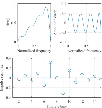
Figure 3.2 Magnitude Response, Passband Error and Impulse Response of Filter Order 𝑁 14 ... 66
Figure 3.3 Minimax Error Convergence Curve of Filter Order 𝑁 14 ... 66
Figure 3.4 Magnitude Response, Passband Error and Impulse Response of Filter Order 𝑁 26 ... 67
Figure 3.5 Minimax Error Convergence Curve of Filter Order 𝑁 26 ... 67
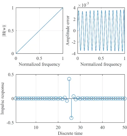
Figure 3.6 Magnitude Response, Passband Error and Impulse Response of Filter Order 𝑁 50 ... 68
Figure 3.7 Minimax Error Convergence Curve of Filter Order 𝑁 50 ... 68
Figure 3.8 Magnitude Response, Passband Error and Impulse Response of Filter Order 𝑁 13 ... 69
Figure 3.9 Minimax Error Convergence Curve of Filter Order 𝑁 13 ... 69
Figure 3.10 Magnitude Response, Passband Error and Impulse Response of Filter Order 𝑁 25 ... 70
Figure 3.11 Minimax Error Convergence Curve of Filter Order 𝑁 25 ... 70
Figure 3.12 Magnitude Response, Passband Error and Impulse Response of Filter Order 𝑁 49 ... 71
xvii
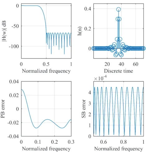
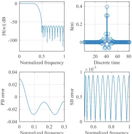
Figure 4.1 Magnitude Response, Impulse Response, Passband and Stopband Errors of Sparse FIR Filter of Order 𝑁 60 ... 82
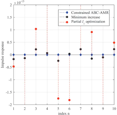
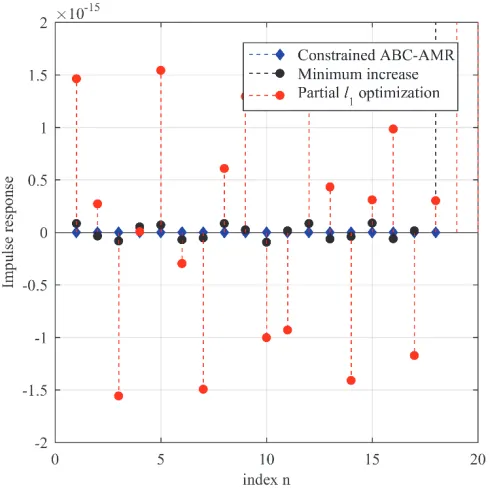
Figure 4.2 Enlarged Impulse Response of Sparse FIR Filter of Order 𝑁 60 ... 83
Figure 4.3 Magnitude Response, Impulse Response, Passband and Stopband Errors of Sparse FIR Filter of Order 𝑁 70 ... 84
Figure 4.4 Enlarged Impulse Response of Sparse FIR Filter of Order 𝑁 70 ... 85
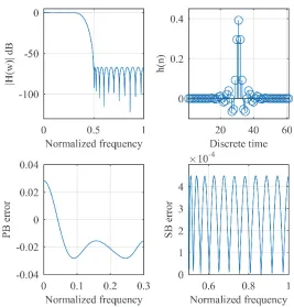
Figure 4.5 Magnitude Response, Impulse Response, Passband and Stopband Errors of Sparse FIR Filter of Order 𝑁 80 ... 86
Figure 4.6 Enlarged Impulse Response of Sparse FIR filter of Order 𝑁 80 ... 87
Figure 5.1 Flowchart of Reference Point-Based MOABC ... 95
Figure 5.2 Magnitude Response, Impulse Response, Passband and Stopband Errors of Asymmetric FIR Lowpass Filter Using MOABC ... 99
Figure 5.3 Magnitude Response, Impulse Response, Passband and Stopband Errors of Asymmetric FIR Lowpass Filter Using MODE ... 99
Figure 5.4 Pareto Front Approximation of Asymmetric FIR Lowpass Filter Using MOABC ... 100
Figure 5.5 Pareto Front Approximation of Asymmetric FIR Lowpass Filter Using MODE ... 100
Figure 5.6 Magnitude Response, Impulse Response, Passband and Stopband Errors of Asymmetric FIR Highpass Filter Using MOABC ... 103
Figure 5.7 Magnitude Response, Impulse Response, Passband and Stopband Errors of Asymmetric FIR Highpass Filter Using MODE ... 103
xviii
Figure 5.9 Pareto Front Approximation of Asymmetric FIR Highpass Filter Using MODE ... 104
Figure 5.10 Magnitude Response, Impulse Response, Passband and Stopband Errors of Asymmetric FIR Bandpass Filter Using MOABC ... 107
Figure 5.11 Magnitude Response, Impulse Response, Passband and Stopband Errors of Asymmetric FIR Bandpass FIR Filter Using MODE ... 107
Figure 5.12 Magnitude Response, Impulse Response, Passband and Stopband Errors of Asymmetric FIR Bandstop Filter Using MOABC... 110
Figure 5.13 Magnitude Response, Impulse Response, Passband and Stopband Errors of Asymmetric FIR Bandstop FIR Filter Using MODE ... 110
Figure 6.1 1S Class Function: Smaller is the Better [190] ... 120
Figure 6.2 Flowchart of Physical-Programming-based MOABC ... 125
Figure 6.3 Magnitude Response, Group Delay Response, Magnitude Errors and Group Delay Errors of IIR Lowpass Filter Designed Using MOABC ... 129
Figure 6.4 Pole Zero Plot of IIR Lowpass Filter Designed Using MOABC ... 129
Figure 6.5 Magnitude Response, Group Delay Response, Magnitude Errors and Group Delay Errors of IIR Highpass Filter Designed Using MOABC ... 132
Figure 6.6 Pole Zero Plot of IIR Highpass Filter Designed Using MOABC ... 133
Figure 6.7 Magnitude Response, Group Delay Response, Magnitude Errors and Group Delay Errors of IIR Bandpass Filter Designed Using MOABC ... 137
xix
LIST OF ACRONYMS
1-D One-Dimensional
2-D Two-Dimensional
ABC Artificial Bee Colony Algorithm
ABC-AMR Artificial Bee Colony Algorithm with Adaptive Modification Rate
CSA Cuckoo Search Algorithm
dB Decibel
DE Differential Evolution
DM Decision Maker
EA Evolutionary Algorithm
FIR Finite Impulse Response
GA Genetic Algorithm
GABC Gbest guided ABC
GME Generalized Multiple Exchange
HSA Harmony Search Algorithm
IEMO Interactive Evolutionary Multiobjective Optimization
IIR Infinite Impulse Response
IRLS Iterative Reweighted Least Squares
LS-MOEA Local Search Operator Enhanced Multiobjective Evolutionary Algorithm
MOABC Multiobjective Artificial Bee Colony
MODE Multiobjective Differential Evolution
xx MOO Multiobjective Optimization
NP Nondeterministic Polynomial time
NSGA Nondominated Sorting Genetic Algorithm
OL Orthogonal Learning
PAES Pareto Archived Evolution Strategy
PM Parks-McClellan
PP Physical Programming
PSO Particle Swarm Optimization
SDP Semidefinite Programming
SOCP Second Order Cone Programming
SPEA Strength Pareto Evolutionary Algorithm
SP Spherical Pruning
1
CHAPTER 1
INTRODUCTION
1.1 Introduction to Digital Filter Design
Electronic filters are circuits capable of passing certain frequency signals to extract useful information. The electronic filters may be analog or digital depending on the components used. The analog filters operate on continuous time analog signals, whereas digital filter performs mathematical operations on digital signals. Unlike analog filters which requires active and passive physical components, the digital filters can be implemented on computers.
Digital filters can be mathematically expressed by the constant coefficient difference equation:
𝑦 𝑛 𝑏 𝑘 𝑥 𝑛 𝑘 𝑎 𝑘 𝑦 𝑛 𝑘 (1.1)
where 𝑏 𝑘 and 𝑎 𝑘 are the forward tap coefficients and feedback tap coefficients respectively. The transfer function of the digital filter can be expressed as,
𝐻 𝑧 𝑌 𝑧
𝑋 𝑧
∑ 𝑏 𝑘 𝑧
1 ∑ 𝑎 𝑘 𝑧 (1.2)
The digital filters can be classified into two categories finite impulse response (FIR) and infinite impulse response (IIR) digital filters depending on the length of their impulse responses and location of poles.
1.1.1 Finite Impulse Response Filters
2 but depends only on the present value of the input. FIR digital filters include asymmetric FIR filters and symmetric FIR digital filters.
The asymmetric FIR filters are a class of causal filters with the difference equation and transfer function is as expressed below,
𝑦 𝑛 𝑏 𝑘 𝑥 𝑛 𝑘 (1.3)
and
𝐻 𝑧 𝑌 𝑧
𝑋 𝑧 𝑏 𝑘 𝑧 (1.4)
The frequency response of filter can be found by substituting 𝑧 𝑒 , where 𝜔 is the frequency of the input signal,
𝐻 𝜔 𝑏 𝑒
𝑏 cos 𝜔𝑛𝑇 𝑗 𝑏 sin 𝜔𝑛𝑇
| 𝐻 𝜔 |𝑒 (1.5)
In equation 1.5, the magnitude response |𝐻 𝑤 |is equal to,
|𝐻 𝑤 | 𝑏 cos 𝑛𝑤𝑇 𝑏 sin 𝑛𝑤𝑇 (1.6)
3
𝜃 𝑤 𝑡𝑎𝑛 ∑ 𝑏 𝑠𝑖𝑛 𝑛𝑤𝑇
∑ 𝑏 𝑐𝑜𝑠 𝑛𝑤𝑇 (1.7)
From equation 1.7, the group delay 𝜏 𝑤 can be expressed as,
𝜏 𝑤 𝜕𝜃 𝑤
𝜕𝑤𝑇
1
1 𝑐
𝜕𝑐
𝜕𝑤𝑇 (1.8)
where,
𝑐 ∑ 𝑏 𝑠𝑖𝑛 𝑛𝑤𝑇
∑ 𝑏 𝑐𝑜𝑠 𝑛𝑤𝑇 (1.9)
The symmetric FIR filters have constant group delay, and the filter coefficients are either symmetric or anti symmetric with respect to mid-point. A filter of order 𝑁 or length 𝑀 𝑁 1 is said to be linear phase if it satisfies the following equation,
ℎ 𝑛 ℎ 𝑀 1 𝑛 (1.10)
where 𝑛 0,1,2, … … … . , 𝑀 1.
Depending on the type of symmetry, there are four types of linear phase FIR filters; Type 1, Type 2, Type 3 and Type 4.
In Type 1 filters, the filter order, 𝑁 𝑀 1 is even and the coefficients are symmetrically distributed,
ℎ 𝑛 ℎ 𝑀 1 𝑛 (1.11)
where 𝑛 0,1,2, … … … . , 𝑀 1 and the frequency response 𝐻 𝜔 is given by,
𝐻 𝜔 𝑒 ℎ 𝑀 1
2 2ℎ 𝑛 cos
𝑀 1
4 In Type 2 filters, the filter order, 𝑁 𝑀 1 is odd and the coefficients are symmetrically distributed,
ℎ 𝑛 ℎ 𝑀 1 𝑛 (1.13)
where 𝑛 0,1,2, … … … . , 𝑀 1 and the frequency response 𝐻 𝜔 is given by,
𝐻 𝜔 𝑒 2ℎ 𝑛 cos 𝑀 1
2 𝑛 𝜔𝑇 (1.14)
In Type 3 filters, the filter order, 𝑁 𝑀 1 is even and the coefficients are anti-symmetrically distributed,
ℎ 𝑛 ℎ 𝑀 1 𝑛 (1.15)
where 𝑛 0,1,2, … … … . , 𝑀 1 and the frequency response 𝐻 𝜔 is given by,
𝐻 𝜔 𝑗𝑒 2ℎ 𝑛 sin 𝑀 1
2 𝑛 𝜔𝑇 (1.16)
In Type 4 filters, the filter order, 𝑁 𝑀 1 is odd and the coefficients are anti - symmetrically distributed,
ℎ 𝑛 ℎ 𝑀 1 𝑛 (1.17)
where 𝑛 0,1,2, … … … . , 𝑀 1 and the frequency response 𝐻 𝜔 is given by,
𝐻 𝜔 𝑗𝑒 2ℎ 𝑛 sin 𝑀 1
5
1.1.2 Infinite Impulse Response Filters
IIR filters include the following; direct-form general IIR filter; direct-form allpass IIR filter; cascade-form general IIR filter and cascade-form allpass IIR filter.
Direct-form general IIR filter consisting of 𝑀th order numerator and 𝑁th order denominator transfer function can be expressed as,
𝐻 𝑧 𝐵 𝑧
𝐴 𝑧
∑ 𝑏 𝑘 𝑧
1 ∑ 𝑎 𝑘 𝑧 𝑐 𝑛 𝑧 (1.19)
where 𝐵 𝑧 and 𝐴 𝑧 are polynomials written in ascending powers of 𝑧 , 𝑀 can be smaller or larger than 𝑁. The coefficients 𝒄 𝑛 for 𝑛 0 represent the impulse response values of the digital filter. The corresponding coefficient vector 𝒄 consisting of 𝑀 𝑁 1 distinct coefficients can be expressed as,
𝒄 𝑏 𝑏 𝑏 … 𝑏 𝑏 𝑎 𝑎 𝑎 … 𝑎 𝑎 (1.20)
Direct-form allpass IIR filter can characterized by a unity magnitude response throughout the frequency band and its group delay response is a function of its coefficient values. It can be used to equalize the group delay of another digital filter or a system connected in cascade. The direct-form transfer function of an 𝑁th-order allpass IIR filter (𝑁 can be even or odd) can be expressed as,
𝐻 𝑧 ∑ 𝑎 𝑧
∑ 𝑎 𝑧 𝑧
∑ 𝑎 𝑧
∑ 𝑎 𝑧 (1.21)
The coefficient vector 𝒄 consisting of 𝑁 1distinct coefficients can be expressed as,
𝒄 𝑎 𝑎 𝑎 … 𝑎 𝑎 (1.22)
6
|𝐻 𝜔 |=1 (1.23)
Cascade-form general IIR filters can be obtained by combining two or more direct-form structures. Assuming both the numerator and denominator transfer function are of same order such that 𝑀 𝑁, the cascade-form transfer function of an even 𝑁th order IIR filter can be expressed as,
𝐻 𝑧 𝑏 𝐵 𝑧
𝐴 𝑧 (1.24)
𝑏 1 𝑏 𝑧 𝑏 𝑧
1 𝑎 𝑧 𝑎 𝑧 𝑐 𝑛 𝑧
where 𝑏 , 𝑏 , 𝑎 ,𝑎 with 𝑛 1 𝑡𝑜 are real valued coefficients, and 𝑏 is a scaling
constant. The coefficients 𝒄 𝑛 for 𝑛 0 represents the impulse response values of IIR filter. The corresponding coefficient vector𝒄 consisting of 2𝑁 1 distinct coefficients can be expressed as,
𝒄 𝑏 𝑏 𝑎 𝑎 … 𝑏 , 𝑏 , 𝑎 , 𝑎 , 𝑏 (1.25)
Cascade-form allpass IIR filter of an even 𝑁 th-order can be expressed as,
𝐻 𝑧 𝑧 1 𝑎 𝑧 𝑎 𝑧
1 𝑎 𝑧 𝑎 𝑧 (1.26)
The corresponding coefficient vector 𝒄 consisting of 𝑁 distinct coefficients can be expressed as,
7 The frequency response of a cascade-form allpass IIR filter can be evaluated by substituting 𝑧 𝑒 into its digital transfer function equation 1.26 and magnitude response is given by,
|𝐻 𝜔 |=1 (1.28)
Two typical classes of design optimization methods for digital filters are and evolutionary optimization [1] and mathematical optimization [2]. A number of useful reference books on digital filter design methods are listed under [3]-[7] and a number of general reference books on digital signal processing are listed in [8]-[10]. A collection of papers on IIR and FIR filter design methods are listed in [11]-[122]. In general, FIR digital filters can be subdivided into linear phase FIR digital filters and nonlinear phase FIR digital filters. The design of linear phase FIR digital filters is described in [11]-[19]; the design of differentiators and integrators are described in [20]-[23]; the design of sparse linear phase FIR digital filters is described in [24]-[46]; and the design of nonlinear phase (or general or asymmetric) FIR digital filters are described in [47]-[60]. An IIR digital filter can be designed to approximate given magnitude response in both passband(s) and stopband(s) and linear phase response in passband(s). The design of IIR digital filters are described in [61]-[85]and adaptive digital filters in [86]-[93]. The design of variable IIR digital filters are described in [94]-110] and variable FIR digital filters is described in [111]. The designs of 2-dimensional FIR digital filters are described in [112]-[114] and IIR digital filters are described in [115]-[122].
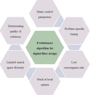
1.2 Limitations of Evolutionary Algorithm in Digital Filter Design
8 Nevertheless, when evolutionary algorithms are used for digital filter design various challenges has been faced, Figure 1.1 shows various limitations of evolutionary algorithm in digital filter design.
Figure 1.1 Limitations of Evolutionary Algorithms in Digital Filter Design
1.2.1 Many Control Parameters and Problem Specific Tuning
Conventional algorithms such genetic algorithm (GA), particle swarm optimization (PSO), and differential evolution (DE) contain many control parameters and each of these parameters must be tuned to their optimal value for best performance. Modifying each of these parameters for filter design application require a tedious task of trial and error run.
9
1.2.2 Low Convergence Rate
Evolutionary algorithms are inspired by the biological process of natural selection and mutation, it is a slow process and needs long computation time to reach global optimum.
1.2.3 Stuck at Local Optima
Even though it is easy to customize the evolutionary algorithms for any application, it is important to choose the best suited algorithm for a given problem. The wrong configuration can lead to premature convergence to a local optimum solution and will not yield global optimum.
1.2.4 Limited Search Space Diversity
In general, for reducing the longer computation time, instead of initializing with a random population, optimization process is seeded with a good candidate solution that is previously known or created. This process is found to reduce the diversity of search space, especially in higher dimension problems.
1.2.5 Deteriorating Quality of Solutions with Increase in Dimensionality
When a limited search space is applied to non-convex, non-differentiable, multimodal, composite functions the quality of solution deteriorates with increase in dimensionality. In filter design applications, peak error value of designed filter cannot be reduced to an optimal value with the increase in filter order.
1.3 Motivation
Classical optimization methods and conventional evolutionary algorithms have certain limitations when applied to digital filter design. In order to overcome these limitations, this dissertation focuses on an improved ABC algorithm for the design of optimal FIR and IIR digital filters.
10 towards any specific problem. However, it faces some difficulties such as lower convergence rate, getting stuck at local optimum and difficulty in minimizing the peak error values of the higher order digital filters. The above said problems are a result of insufficient balance between the exploration and exploitation in the search equation. Exploration refers to investigating unknown regions in the solution space to discover global optimum and exploitation refers to applying knowledge about previous good solution to find a better solution. The former occurs at initial stages of optimization while latter at later stages of optimization. Though these two techniques contradict each other, a proper balance between them is necessary for obtaining optimal results. Many variants of ABC algorithm have been developed to address the concerning issues, most of them improves the exploitation by directing the search towards the best solution, but this will limit the diversity in the search space. As filter design problem is analyzed, in order to lower peak error value and satisfy design constraints of higher order filters, new solutions must be introduced into the solution space. So, in this dissertation, a novel improvement known as adaptive modification rate is introduced to the original ABC algorithm, which mutates the parameters in the solution space adaptively.
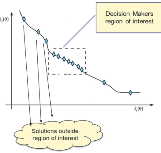
11 guide the search toward the region of interest. Different approaches can be used to incorporate the decision maker’s preferences into the optimization process. In a posteriori methods, preferences can be used at the end after Pareto front has been completely determined whereas in a priori methods, preferences are given at the beginning of search process which requires the decision maker to have some high-level information about the objectives initially. Interactive methods involve the preferences to be set up interactively during the optimization process.
In this dissertation, the preferences are incorporated into multiobjective optimization a priori by physical programming approach and reference point-based approach.
1.4 Main Contributions
Digital filter design is an approximation problem, in which a designer tries to find a set of filter coefficients which provides the best approximation of a desired filter. Even though, it is impossible to produce exact magnitude or phase response of desired filter the classical methods such as Butterworth and Chebyshev methods can be applied for the design of optimal basic filters. Design of filters with arbitrary magnitude and phase response can only be formulated as complex approximation problem and can be solved using evolutionary algorithms. Using ABC algorithm, improved ABC algorithms and ABC-AMR algorithm, various digital filters are designed in both single-objective space and multiobjective space. The main contributions are listed below:
The dissertation provides an in-depth analysis of ABC algorithm based digital filter design, its advantages, limitations and modifications to be applied for improving its performance in filter design. Initially, an investigation has been performed into the modifications available in the literature. Various digital filters are designed using basic ABC algorithm, its variants and their error values have been compared.
12 differentiators using artificial bee colony algorithm,” in Proc. of 8th International Conference on Wireless Communications and Signal Processing (WCSP 2016), Yangzhou, China, Oct. 13-15, 2016, pp. 1-4. Simulation results indicate that the proposed method can be used successfully to design various digital filters.
In order to minimize hardware requirement in filter design problems, another class of digital filters known as sparse filters are designed using constrained ABC-AMR algorithm and iterative shrinkage technique. The work has been published in - R. Raju, H. K. Kwan and A. Jiang, “Sparse FIR filter design using artificial bee colony algorithm,” in Proc. of IEEE 61st International Midwest Symposium on Circuits and Systems (MWSCAS 2018), Windsor, Ontario, Canada, Aug. 2018, pp. 956-959. Using constrained ABC-AMR algorithm, an increase in sparsity of digital filter can be achieved. Sparse digital filters can be used in applications where computational cost and hardware complexities are critical, because located sparse or zero-valued coefficients do not require multiplications.
For designing asymmetric FIR filters in a multiobjective space, a user can provide a reference point and the search can be directed towards preferred regions in the Pareto front by minimizing the normalized Euclidean distance towards the reference point. Using the reference-point-based multiobjective ABC, asymmetric FIR filters are designed, and the work has been published in - R. Raju and H. K. Kwan, “FIR filter design using multiobjective artificial bee colony algorithm,” in Proc. of 2017 IEEE 30th Canadian Conference on Electrical and Computer Engineering (CCECE 2017), Windsor, Ontario, Canada, Apr. 30-May 3, 2017, pp. 1-4. Comparing the obtained design results with those obtained by the multiobjective differential evolution, lower error values can be obtained.
13 different degrees of desirability such as highly desirable (HD), desirable (D), tolerable (T), undesirable (U) and highly undesirable (HU). Solutions in undesirable (U) and highly undesirable (HU) are not considered in the optimization process. Using a physical programming method, IIR filters are designed and the work has been published in - R. Raju and H. K. Kwan, “IIR filter design using multiobjective artificial bee colony algorithm,” in Proc. of 2018 IEEE 31th Canadian Conference on Electrical and Computer Engineering (CCECE 2018), Quebec City, Quebec, Ontario, Canada, May 13-16, 2018, pp. 1-4.The proposed design method can achieve similar or better results when compared to state-of-the-art design methods.
1.5 Organization
14
CHAPTER 2
LITERATURE SURVEY
Evolutionary algorithms (EA) are population-based metaheuristic search methods that imitate the processes of Darwinian Evolution. Given a set of potential solutions, evolutionary algorithms apply the principle of survival of the fittest to discover optimal solutions in a search space. New individuals in each generation are created by selecting the parent individuals from the existing population according to their level of fitness and by applying principle of natural genetics. This process will improve the quality of individuals in each generation and finally evolve to an optimal solution.
Evolutionary algorithms are inspired by natural process such as reproduction, selection, recombination and mutation. Every individual in the population represents a single possible solution of the optimization problem. EA starts with a set of randomly initialized population. Fitness value of the solutions is calculated by evaluating the objective function for every individual. The individuals with higher fitness value represent the better-quality solutions and some of these individuals are chosen to seed the next generation by applying recombination or mutation. If optimization criteria or maximum number of generations are not met, new generation will be started to produce a new set of individuals. Recombination is an operator in which two or more selected individuals are combined to produce one or more offsprings. Each offspring is then mutated, and its fitness value is calculated. If a new offspring is better than its parents, it is inserted into the current population producing an individual in a new generation. This new generation becomes the current population and the iterative process repeats until it reaches the optimum solution.
15 Holland and Goldberg [123]-[124]; particle swarm optimization (PSO) by Kennedy and Eberhart [125]; ant colony optimization (ACO) by Dorigo and Stutzle [126]; differential evolution (DE) by Storn and Price [127]; simulated annealing by Kirkpatrick et al. [128].
2.1 Artificial Bee Colony Algorithm (ABC)
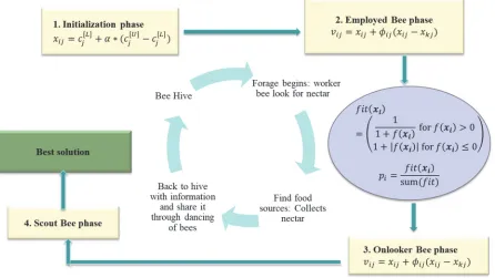
The ABC algorithm is metaheuristic optimization algorithm defined by Dervis Karaboga in 2005 [129], based on collective intelligent biological behavior of honey bee colonies.
Figure 2.1 Schematic Representation of Foraging Behavior of Honey Bees
16 dances to communicate important messages. “Waggle dance” is performed by a worker bee back at the hive to tell other bees about where to find food sources. The dance shows the direction of flowers relative to the sun, and bees automatically adjust their dances according to changing position of the sun. Speed of the dance indicates how far nectar is from the hive.
Inspired by the foraging behavior of honey bee colonies, Karaboga proposed the ABC algorithm [129]-[133] to solve multimodal, multidimensional problems. The foraging behavior of honey bees and a schematic diagram for the ABC algorithm is shown in Figure 2.1. Unlike other optimization algorithms, the ABC algorithm does not need any parameter tuning. The ABC algorithm finds the best solution in a search space like worker bees in bee hives searching for food sources with the highest amount of nectar. In contrast to other heuristic search algorithms, the ABC algorithm showed superior performance and has several advantages: strong robustness, fast convergence, high flexibility and fewer control parameters. Search strategy of the ABC algorithm is like the standard DE algorithm; however, it has a decision making mechanism that decides which areas within the search space is required to be surveyed in detail. This strategy discovers new high quality nectar sources within a search space while preserving existing good quality solutions.
The ABC contains three groups: scouts, onlooker bees, and employed bees [129]-[133]. A bee carrying out the random search is a scout. A bee going to the food source which has been visited previously is called an employee bee. A bee waiting in the dance area is called an onlooker bee. The number of food sources is equal to the number of employed or onlooker bees. A solution which cannot be improved after several predetermined trials becomes a scout bee and is abandoned. The best food source indicates a promising solution to an optimization problem and a fitness function is used to evaluate the quality of the solution obtained.
17
2.1.1 Initialization Phase
In initialization phase of the ABC algorithm, initial food locations are generated as a uniform random distribution, total number of food locations 𝑆𝑁 is equal to the number of employed bees or onlooker bees,
𝒙 𝒙 , 𝒙 , 𝒙 , … , 𝒙 , 𝒙 (2.1)
where 𝒙𝒊 for 𝑖 1 to 𝑆𝑁is a 1 𝐷 vector generated as,
𝑥 𝑐 α 𝑐 𝑐 (2.2)
where α is a random number in 0,1 , 𝑗 ∈ 1,2, … … … . 𝐷 , 𝑐 and 𝑐 are the upper and
lower limits of 𝑗th dimension. Each food location is associated with an employed bee which exploits current location to find a better food location in its neighborhood.
2.1.2 Employed Bee Phase
In employed bee phase, bees search iteratively for food within a population. An employed bee first searches for foods in the adjacent region of its current food source, a new food location 𝒗 is calculated by,
𝑣 𝑥 𝜙 𝑥 𝑥 (2.3)
where 𝑗 is a randomly selected parameter index; 𝒙 is a randomly selected food source; ϕ
is a random number within the range [-1,1]. If the fitness value of new food source is better than current one, then current food source is replaced by new food source. The fitness value is calculated using equation,
𝑓𝑖𝑡 𝒙
1
1 𝑓 𝒙 for 𝑓 𝒙 0
1 |𝑓 𝒙 | for 𝑓 𝒙 0
(2.4)
18
2.1.3 Onlooker Bee Phase
When employed bees complete their food search, they pass the information to onlooker bees which in turn choose their food sources depending on the probability value calculated using,
𝑝 𝑓𝑖𝑡 𝒙
∑ 𝑓𝑖𝑡 𝒙 (2.5)
where 𝑓𝑖𝑡 𝒙 is the fitness value associated with food location and is given by equation 2.4. Solutions with a higher fitness value has a greater probability of being chosen by onlooker bees.
2.1.4 Scout Bee Phase
In scout bee phase, a food source that is not improved after several trials, will be changed to a scout bee. Scout bees will randomly search for a new solution according to equation 2.2.
Numerical comparison of the ABC algorithm with other swarm-based algorithms [131]-[133], indicate that former can produce better results with benefit of fewer control parameters. A review of the ABC algorithm can be found in [134]. As the ABC algorithm is free from parameter tuning it is used widely in a variety of practical applications.
Like other evolutionary algorithms, the ABC algorithm also faces shortcomings such as getting trapped in local minima, and slower convergence speed. The above two problems are a result of insufficient balance between exploration and exploitation capability of search equation in the ABC algorithm. The solution generation equation which produces new food source based on the information of the previous solution, is good at exploration but poor in exploitation. Accelerating convergence speed and avoiding local optima are two most important goals in the ABC research.
19 exploitation. To address this concerning issue, numerous ABC variants have been developed. These improvements can be divided into two types, primarily new solution search equations have been introduced and secondarily, the original ABC is hybridized with other techniques. Some of the most popular modifications of the ABC algorithm are described below.
The ABC algorithm in its original version lacks a mechanism to deal with constrained optimization problems. Hence, a number of modifications have been applied to the original ABC algorithm to improve its performance for specific constrained engineering application problems. For constraint handling, the ABC algorithm can be combined with the Deb’s rule and a probabilistic selection scheme to determine the optimum solution in the feasible region of a search space depending on a violation index value [135]. The first modification is made in the solution generation equation in employed and onlooker bee phase by changing more than one parameter in each iteration. In the second modification, greedy selection in the ABC algorithm is replaced by the Deb’s selection mechanism which assigns probability value to solutions based on their fitness value. The probability value for each solution is generated according to the following equation,
𝑝
⎩ ⎪ ⎨ ⎪
⎧0.5 ∑ 𝑓𝑖𝑡 𝒙𝑓𝑖𝑡 𝒙 0.5 if solution is feasible
1 ∑ 𝑣𝑖𝑜𝑙𝑎𝑡𝑖𝑜𝑛
𝑣𝑖𝑜𝑙𝑎𝑡𝑖𝑜𝑛 0.5 otherwise
(2.6)
where 𝑣𝑖𝑜𝑙𝑎𝑡𝑖𝑜𝑛, is the penalty value of the solution 𝒙 and 𝑓𝑖𝑡 𝒙 is the fitness value of the solution 𝒙 . Probability values of infeasible solutions are between 0 and 0.5 while those of feasible ones are between 0.5 and 1. By a selection mechanism like roulette wheel, solutions are selected probabilistically proportional to their fitness values of feasible solutions and inversely proportional to their violation values of infeasible solutions.
20
𝑣 𝑥 𝜙 𝑥 𝑥 𝜑 𝑥 , 𝑥 𝑖 𝑘 (2.7)
where 𝑥 , is a randomly selected parameter index of global best solution, 𝒙 is
randomly selected food source, ϕ is a random number within the range [-1,1], 𝜑 ∈
0, 𝐶 where C is a constant. The value of C is determined through the trial and error method by applying it on different benchmark functions.
Diwold et al. [137] proposed a variation to the gbest-guided ABC algorithm, where a random neighbor selection is controlled through the following equation. Let 𝑑 𝒙 , 𝒙 be the Euclidean distance between two solutions 𝒙 and 𝒙 , the solution 𝒙 will be chosen with probability defined by,
𝑝
1 𝑑 𝒙 , 𝒙
∑ , 𝑑 𝒙 , 𝒙1 (2.8)
The closer solution has greater probability of being selected. The idea behind this modification is that it is more probable to find a better solution by mutating two good solutions close to each other in a solution space.
The best-so-far selection ABC algorithm [138] exploits the best solution found so far to improve convergence speed of the original ABC algorithm. The employed bee phase is unaltered as in equation 2.2, while onlooker bee phase is changed as follows,
𝑣 𝑥 𝑓𝑖𝑡 𝜙 𝑥 𝑥 , 𝑖 𝑘, 𝑑 1,2 … … 𝐷 (2.9)
where 𝑗 is a randomly selected dimension, and 𝑓𝑖𝑡 is the fitness value of the best
21
𝑥 𝑥 𝑥 ∗ 𝜙 𝑤 𝑖𝑡𝑒𝑟
𝑖𝑡𝑒𝑟 𝑤 𝑤 (2.10)
where 𝑗 ∈ 1, 𝐷 , 𝑤 , 𝑤 are control parameters to determine the strength of perturbation and is fixed as 1 and 0.2 respectively, 𝑖𝑡𝑒𝑟 is current iteration number and 𝑖𝑡𝑒𝑟 is maximum number of iterations. As per the above equation, as number of iterations increases, algorithm is more exploitative than explorative.
Alatas [139] proposed two new chaotic ABC algorithm by using seven different chaotic maps as random number generators to improve convergence characteristics and to prevent the ABC algorithm from getting stuck at local solutions. In the chaotic ABC 1, instead of using uniform random distribution for population initialization it uses a chaotic map to
generate solutions. In the chaotic ABC 2, if a solution cannot be improved after trials,
algorithm starts chaotic search for trials around current solution by modifying the
dimension and accepts new solution if it improves the current one. By combing modifications of the chaotic ABC 1 and the chaotic ABC 2, another variant of the ABC algorithm called the chaotic ABC 3 is proposed.
In an improved ABC algorithm [140], the population is initialized using chaotic random generator-based on the logistic map. After generating 𝑆𝑁 solutions randomly, a new set of 𝑆𝑁 solutions are generated by opposition-based population initialization, in which each variable is mirrored at the center of search range. From 2 ∗ 𝑆𝑁 solutions the best 𝑆𝑁 solutions are kept. Also, it modifies the search mechanism in onlooker and employed bee phases by incorporating differential evolution-based search. It uses following two equations inspired by the DE/best/1 and the DE/rand/1 scheme respectively,
In the ABC/best/1, equation 2.3 is modified as,
𝑣 𝑥 , 𝜙 𝑥 𝑥 , (2.11)
22
𝑣 𝑥 , 𝜙 𝑥 𝑥 , (2.12)
where 𝑟1 and 𝑟2 are two random indices different from 𝑖, 𝑥 , is the 𝑗 dimension
randomly chosen from the best solution found so far. In the above equations, equation 2.11 biases a search towards the best solution in the current population which can improve convergence speed but may lead to a premature convergence, whereas equation 2.12 utilizes explorative property to prevent premature convergence. The above two equations are combined to find a new hybridized ABC search mechanism in which, a selective probability 𝑝 is used to control the frequency of introducing the ABC/best/1 and the ABC/rand/1. The value of selective probability 𝑝 is set as 0.25.
Inspired by the differential evolution, Gao. et al. [140]-[141] proposed the global best ABC algorithm in which a solution search in employed and onlooker looker bee phases is directed towards the best solution of the previous iteration. Initial population is generated using a chaotic system and opposition-based learning which possesses ergodicity, randomness and irregularity to generate initial populations. Sinusoidal iterator is selected, and its equation is defined as follows,
𝑐ℎ sin 𝜋𝑐ℎ 𝑐ℎ 𝜖 0,1 , 𝑘 0,1,2 … … … . 𝐾 (2.13)
Based on variants from the differential evolution, the employed and onlooker bee phases are modified in the ABC/best/1 as follows,
𝑣 𝑥 , 𝜙 𝑥 , 𝑥 , (2.14)
and in the ABC/best/2 as follows,
𝑣 𝑥 , 𝜙 𝑥 , 𝑥 , 𝜙 𝑥 , 𝑥 , (2.15)
23 number in range 1,1 . In equation 2.3, the coefficient 𝜙 is a uniform random number
in [−1, 1] and 𝑥 is a random individual in population, and therefore, a solution search
dominated by equation 2.3 is random enough for exploration. However, according to equation 2.14 or equation 2.15, ABC/best can drive a new candidate solution around the best solution of the previous iteration. Therefore, modified solution search equation described by above equation can increase exploitation of the ABC algorithm.
In the Rosenbrock ABC algorithm [142], optimization is carried out in two phases, during exploration phase, the ABC algorithm locates regions of attraction and during exploitation phase, it uses the adaptive Rosenbrock’s rotational direction method to carry out a local search near the best solution.
In the first modification, fitness function is modified as follows,
𝑓𝑖𝑡 2 𝑆𝑃 2 𝑆𝑃 1 𝑟 1
𝑆𝑁 1 (2.16)
where 𝑆𝑃 ∈ 1.0,2.0 is a parameter called selection pressure, 𝑟 is rank of solution of 𝒙 in the population. In the second modification, for every 𝑛 cycles of the ABC, a local search technique, the Rosenbrock’s rotational direction method, is initiated with the global best solution as a starting point. An adaptive step size 𝛿, is defined as a fraction of average distance between selected solutions and the best solution achieved so far and is determined by following equation,
𝛿 0.1∑ 𝑥 𝑥 ,
𝑚 (2.17)
where 𝛿 is step size of 𝑗th dimension, 𝑚 is the first 10% of solutions used to calculate step
24 In the incremental ABC [143] with local search method, a new population is added to the initial population after every 𝑔 iterations, biased by the members of a current population. The employed and onlooker bee phases are modified as follows,
𝑣 𝑥 𝜙 𝑥 , 𝑥 (2.18)
The scout bee phase is initialized by biasing towards the global best solution as,
𝑥 𝑥 , 𝑅 𝑥 , 𝑥 , (2.19)
where 𝑥 is a new solution replacing an abandoned solution and 𝑅 is the bias towards
the global best solution. When population size is increased, equation 2.3 of the employed bee phase is replaced as follows,
𝑣 , 𝑥 , 𝜙 𝑥 , 𝑥 , (2.20)
where 𝑥 , is generated using equation 2.3, 𝑣 is the 𝑗th coordinate biased by the
global best solution, and 𝜙 is a random parameter.
In the orthogonal learning-based ABC algorithm [144], a new search equation is used in the employed and onlooker bee phases as,
𝑣 𝑥 , 𝜙 𝑥 , 𝑥 , (2.21)
where 𝑟, and 𝑟 are mutually exclusive integers randomly chosen from 𝑆𝑁 food locations and different from base index 𝑖, and 𝜙 is the random number in the range 1,1 . In
equation 2.21, the vectors for generating candidate solutions are selected from the population randomly. Consequently, it has no bias in any search direction. As it is guided
of only one term 𝜙 𝑥 , 𝑥 , , it can easily avoid oscillation phenomenon and
25 strategy-based algorithm (OCABC), combines the ABC algorithm with OL, the transmission vector 𝑻 is generated as follows,
𝑻 𝒙 𝑟𝑎𝑛𝑑 0,1 𝒙 𝒙 (2.22)
𝑻 and 𝒙 are mixed by making use of the orthogonal learning strategy to obtain a new solution 𝒗 , and a greedy selection is applied to select the best solution for the next generation.
In the Gaussian-based ABC algorithm [145], the food search equations in the employed and onlooker bee phases are updated as follows,
𝑥 𝑥 ∆.2 𝑟 0.5 𝛽𝛼 𝑖𝑓 𝑟 𝑝
𝑥 𝑥 ∆.2 𝑟 0.5 2𝛼 𝑖𝑓 𝑟 𝑝
(2.23)
where 𝑟, 𝑟 ϵ 0,1 are random numbers from uniform distribution,
∆ 𝑥 𝑥
𝛽 |𝑠|
𝛼 0.5 0.25 𝑖𝑡𝑒𝑟 𝑚𝑎𝑥𝑖𝑡𝑒𝑟
(2.24)
where 𝑠 is a random number extracted from a gaussian (normal) distribution and 𝑖𝑡𝑒𝑟 and 𝑚𝑎𝑥𝑖𝑡𝑒𝑟 indicate current iteration and maximum iteration number respectively; 𝑝 is responsible for a balance between gaussian and uniform distribution, and smaller values of 𝑝 seem preferable, indicating a superiority of the gaussian distribution. This method improves the performance of the ABC algorithm through a better balance between exploration and exploitation of the search space.
26 two search mechanisms are designed to facilitate an exchange of information in each subpopulation and between different subpopulations. In the employed bee phase, the search equation is updated with the 𝑙𝑏𝑒𝑠𝑡 individual as,
𝑡 𝐹 . 𝑥 , 𝐹 . 𝑥 ,
𝐹 𝐹
𝑣 𝑡 ∅ 𝑡 𝑥 ,
(2.25)
In the onlooker bee phase, the search equation is updated with the 𝑔𝑏𝑒𝑠𝑡 individual as,
𝑡 𝐹 . 𝑥 , 𝐹 . 𝑥 ,
𝐹 𝐹
𝑣 𝑡 ∅ 𝑡 𝑥 ,
(2.26)
where 𝑗 𝜖 1, … . 𝐷 and ∅ is a random number in 1,1 ; 𝑘1 and 𝑘2 are randomly
selected indices in 1, 𝑆𝑁 such that 𝑘1 𝑘2 𝑖; 𝑙𝑏𝑒𝑠𝑡 and 𝑔𝑏𝑒𝑠𝑡 are the indices of the best individuals found by corresponding subpopulation and whole population respectively; 𝑻𝒊 is a transmission vector; 𝐹𝑟 is fitness ranking of the 𝑖th individual in the current whole population from worst to best. Introduction of information about 𝑙𝑏𝑒𝑠𝑡 and 𝑔𝑏𝑒𝑠𝑡 in the search equations can guide the search towards promising regions and speed up convergence. Thus, the two search mechanisms have stronger exploitation than the original ABC. On the other hand, the information of a randomly selected individual 𝒙 in the neighborhood is inserted into the transmission vector which can maintain population diversity and escape from trapping into local optimum.
27 also hybridized with the genetic algorithm [148]-[149] and the particle swarm optimization [150]-[153]. Inspired by foraging behavior of bacteria, Zhong et al. [154], introduced a local search technique in solution update equations of employed and onlooker bee phase. The differential evolution[155] and a chaotic operator [156] have been introduced into the search equation of the original ABC algorithm to improve its convergence speed. For improving movement of a scout bee, mechanisms based on nonlinear interpolated path and gaussian movement is proposed by Sharma and Pant [157]. To improve solution search equation, Rajasekhar et al. [158] introduced levy probability distributions. The improved artificial bee colony algorithm [159] with a new search cycle operator is used to solve higher dimensional multimodal problems. Tsai et al. [160] proposed the interactive ABC algorithm in which a gravitational force is used to drive the bee movement in onlooker phase. The hybrid simplex ABC algorithm was proposed by Kang et al. [161]by integrating the Nelder-mead simplex method into the ABC algorithm. A hybrid swarm intelligent approach based on the genetic algorithm and the ABC algorithm was proposed by Zhao et al. [162], which combines the parallel computation merit of the genetic algorithm with the self-improving ability of the ABC Algorithm by exchanging information between bee colony and genetic algorithm population. An improved quantum EA was proposed by Duan et al. [163] which uses the ABC algorithm to improve the local search ability and escape from trapping into the local optima. The ABC algorithm have also been hybridized with the Hooke-jeeves pattern search [164] and the Powell’s method [165] to improve its exploitation capability.
28
2.2 Challenges Faced by Variants of ABC Algorithm in Digital Filter Design
The modifications to the original ABC algorithm, in general, improves exploitation capability of the search equation but various challenges are faced when they are applied to digital filter design. Some of them are listed in Figure 2.2.
2.2.1 Strong Impact of Local Search and Directed Search
A local search method can improve the performance of continuous optimization in many population-based metaheuristics. Generally, a local search is applied with an initial point as the global best solution and finds whether a local search can replace the best solution obtained so far. Trade-off between local search and global search is essential for successful optimization, because if the effect of local search is too strong then the ABC algorithm-based optimization is insignificant. Also, in many variants of the ABC algorithm, exploitation of search equation is improved by directing the search towards the best solution obtained so far, which increases the chance of getting stuck at a local optimum and decreases the quality of solutions for higher dimensional problems.
29
2.2.2 Issues in Obtaining a Global Optimum Solution
Directing the search towards the best solutions in the solution space makes variables in all dimensions comes closer. These types of algorithms can be used to solve problems which has same optimum value in all dimensions like 𝑓 𝒙 0,0, … … … … 0 . In some
variants of the ABC algorithm, their solution update equations are applied to all dimensions [138], instead of a single dimension in every iteration. In such cases the variables in each dimension will have optimum value in different directions, guiding the search towards the best solution will restrict the search in the multi directions, which increases the error value and, deteriorates the optimization performance.
2.2.3 Hybrid ABC
In addition to incorporating the ABC algorithm with local search heuristics [147], the search equation can be updated by incorporating other evolutionary algorithm such as the GA [148]-[149], the PSO [150]-[151] into the ABC algorithm. This will improve the performance in some benchmark functions, but it requires tuning of the control parameters of each of these evolutionary algorithms, which in turn increases the computational cost.
2.2.4 Diversity of Search Space
Directing a search towards the best solution will increase exploitation but limits the diversity of a search space. When the search is biased towards the neighborhood of best solution, it limits exploration of unknown regions in a search space and restricts the diversity of a population.
2.3 Multiobjective Optimization
Many multiobjective algorithms have been developed in the past decade to deal with optimization problems involving more than one objective. In general, a multiobjective optimization problem can be stated [166] as,