multireg.pdf

Full text

(1)C8057 (Research Methods in Psychology): Multiple Regression . Multiple Regression Using SPSS The following sections have been adapted from Field (2009) Chapter 7. These sections have been edited down considerably and I suggest (especially if you’re confused) that you read this Chapter in its entirety. You will also need to read this chapter to help you interpret the output. If you’re having problems there is plenty of support available: you can (1) email or see your seminar tutor (2) post a message on the course bulletin board or (3) drop into my office hour. . What is Correlational Research? Correlational designs are when many variables are measured simultaneously but unlike in an experiment none of them are manipulated. When we use correlational designs we can’t look for cause-‐effect relationships because we haven’t manipulated any of the variables, and also because all of the variables have been measured at the same point in time (if you’re really bored, Field, 2009, Chapter 1 explains why experiments allow us to make causal inferences but correlational research does not). In psychology, the most common correlational research consists of the researcher administering several questionnaires that measure different aspects of behaviour to see which aspects of behaviour are related. Many of you will do this sort of research for your final year research project (so pay attention!). This handout looks at such an example: data have been collected from several questionnaires relating to clinical psychology, and we will use these measures to predict social anxiety using multiple regression. . The Data Anxiety disorders take on different shapes and forms, and each disorder is believed to be distinct and have unique causes. We can summarise the disorders and some popular theories as follows: •. Social Anxiety: Social anxiety disorder is a marked and persistent fear of 1 or more social or performance situations in which the person is exposed to unfamiliar people or possible scrutiny by others. This anxiety leads to avoidance of these situations. People with social phobia are believed to feel elevated feelings of shame. . •. Obsessive Compulsive Disorder (OCD): OCD is characterised by the everyday intrusion into conscious thinking of intense, repetitive, personally abhorrent, absurd and alien thoughts (Obsessions), leading to the endless repetition of specific acts or to the rehearsal of bizarre and irrational mental and behavioural rituals (compulsions). . Social anxiety and obsessive compulsive disorder are seen as distinct disorders having different causes. However, there are some similarities. •. They both involve some kind of attentional bias: attention to bodily sensation in social anxiety and attention to things that could have negative consequences in OCD. . •. They both involve repetitive thinking styles: social phobics are believed to ruminate about social encounters after the event (known as post-‐event processing), and people with OCD have recurring intrusive thoughts and images. . •. They both involve safety behaviours (i.e. trying to avoid the thing that makes you anxious). . This might lead us to think that, rather than being different disorders, they are just manifestations of the same core processes. One way to research this possibility would be to see whether social anxiety can be predicted from measures of other anxiety disorders. If social anxiety disorder and OCD are distinct we should expect that measures of OCD will not predict social anxiety. However, if there are core processes underlying all anxiety disorders, then 1 measures of OCD should predict social anxiety . 1. Those of you interested in these disorders can download my old lecture notes on social anxiety (http://www.statisticshell.com/panic.pdf) and OCD (http://www.statisticshell.com/ocd.pdf). . © Professor Andy Field, 2008 . . Page 1 .

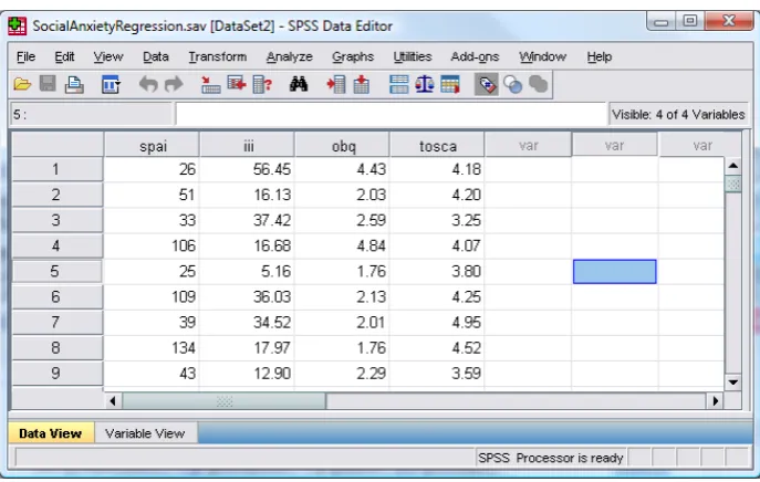
(2) C8057 (Research Methods in Psychology): Multiple Regression The data for this handout are in the file SocialAnxietyRegression.sav which can be downloaded from the course website. This file contains four variables: •. The Social Phobia and Anxiety Inventory (SPAI), which measures levels of social anxiety. . •. Interpretation of Intrusions Inventory (III), which measures the degree to which a person experiences intrusive thoughts like those found in OCD. . •. Obsessive Beliefs Questionnaire (OBQ), which measures the degree to which people experience obsessive beliefs like those found in OCD. . •. The Test of Self-‐Conscious Affect (TOSCA), which measures shame. . Each of 134 people was administered all four questionnaires. You should note that each questionnaire has its own column and each row represents a different person (see Figure 1). The data in this handout are deliberately quite similar to the data you will be analysing for Autumn Portfolio assignment 2. The Main difference is that we have different variables. . Figure 1: Data layout for multiple regression . What analysis will we do? We are going to do a multiple regression analysis. Specifically, we’re going to do a hierarchical multiple regression analysis. All this means is that we enter variables into the regression model in an order determined by past research and expectations. So, for your analysis, we will enter variables in so-‐called ‘blocks’: •. Block 1: the first block will contain any predictors that we expect to predict social anxiety. These variables should be entered using forced entry. In this example we have only one variable that we expect, theoretically, to predict social anxiety and that is shame (measured by the TOSCA). . •. Block 2: the second block will contain our exploratory predictor variables (the one’s we don’t necessarily expect to predict social anxiety). This bock should contain the measures of OCD (OBQ and III) because these variables shouldn’t predict social anxiety if social anxiety is indeed distinct from OCD. These variables should be entered using a stepwise method because we are ‘exploring them’ (think back to your lecture). . . © Professor Andy Field, 2008 . . Page 2 .

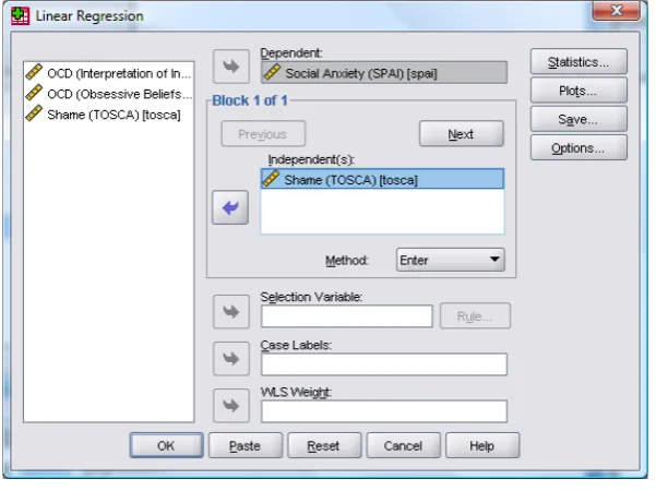
(3) C8057 (Research Methods in Psychology): Multiple Regression . Doing Multiple Regression on SPSS Specifying the First Block in Hierarchical Regression Theory indicates that shame is a significant predictor of social phobia, and so this variable should be included in the model first. The exploratory variables (obq and iii) should, therefore, be entered into the model after shame. This method is called hierarchical (the researcher decides in which order to enter variables into the model based on past research). To do a hierarchical regression in SPSS we enter the variables in blocks (each block representing one step in the hierarchy). To get to the main regression dialog box select select . The main dialog box is shown in Figure 2. . Figure 2: Main dialog box for block 1 of the multiple regression The main dialog box is fairly self-‐explanatory in that there is a space to specify the dependent variable (outcome), and a space to place one or more independent variables (predictor variables). As usual, the variables in the data editor are listed on the left-‐hand side of the box. Highlight the outcome variable (SPAI scores) in this list by clicking on it and then transfer it to the box labelled Dependent by clicking on or dragging it across. We also need to specify the predictor variable for the first block. We decided that shame should be entered into the model first (because theory indicates that it is an important predictor), so, highlight this variable in the list and transfer it to the box labelled Independent(s) by clicking on or dragging it across. Underneath the Independent(s) box, there is a drop-‐down menu for specifying the Method of regression (see Field, 2009 or your lecture notes for multiple regression). You can select a different method of variable entry for each block by clicking on , next to where it says Method. The default option is forced entry, and this is the option we want, but if you were carrying out more exploratory work, you might decide to use one of the stepwise methods (forward, backward, stepwise or remove). Specifying the Second Block in Hierarchical Regression Having specified the first block in the hierarchy, we move onto to the second. To tell the computer that you want to specify a new block of predictors you must click on . This process clears the Independent(s) box so that you can enter the new predictors (you should also note that above this box it now reads Block 2 of 2 indicating that you are in the second block of the two that you have so far specified). We decided that the second block would contain both of the new predictors and so you should click on obq and iii in the variables list and transfer them, one by one, to the Independent(s) box by clicking on . The dialog box should now look like Figure 3. To move between blocks use the and buttons (so, for example, to move back to block 1, click on ). . © Professor Andy Field, 2008 . . Page 3 .

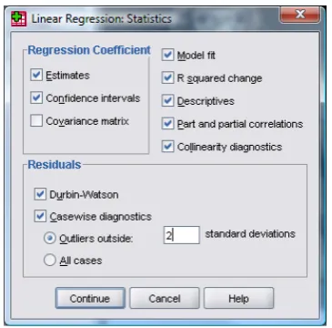
(4) C8057 (Research Methods in Psychology): Multiple Regression It is possible to select different methods of variable entry for different blocks in a hierarchy. So, although we specified forced entry for the first block, we could now specify a stepwise method for the second. Given that we have no previous research regarding the effects of obq and iii on SPAI scores, we might be justified in requesting a stepwise method for this block (see your lecture notes and my textbook). For this analysis select a stepwise method for this second block. . Figure 3: Main dialog box for block 2 of the multiple regression . . Statistics In the main regression dialog box click on to open a dialog box for selecting various important options relating to the model (Figure 4). Most of these options relate to the parameters of the model; however, there are procedures available for checking the assumptions of no multicollinearity (Collinearity diagnostics) and independence of errors (Durbin-‐ Watson). When you have selected the statistics you require (I recommend all but the covariance matrix as a general rule) click on to return to the main dialog box. . . Figure 4: Statistics dialog box for regression analysis → Estimates: This option is selected by default because it gives us the estimated coefficients of the regression model (i.e. the estimated b-‐values). Test statistics and their significance are produced for each regression 2 coefficient: a t-‐test is used to see whether each b differs significantly from zero. → Confidence intervals: This option, if selected, produces confidence intervals for each of the unstandardized regression coefficients. Confidence intervals can be a very useful tool in assessing the likely value of the regression coefficients in the population. → Model fit: This option is vital and so is selected by default. It provides not only a statistical test of the model’s ability to predict the outcome variable (the F-‐test), but also the value of R (or multiple R), the corresponding 2 2 R , and the adjusted R . 2 → R squared change: This option displays the change in R resulting from the inclusion of a new predictor (or block of predictors). This measure is a useful way to assess the unique contribution of new predictors (or blocks) to explaining variance in the outcome. . 2. Remember that for simple regression, the value of b is the same as the correlation coefficient. When we test the significance of the Pearson correlation coefficient, we test the hypothesis that the coefficient is different from zero; it is, therefore, sensible to extend this logic to the regression coefficients. . © Professor Andy Field, 2008 . . Page 4 .

(5) C8057 (Research Methods in Psychology): Multiple Regression → Descriptives: If selected, this option displays a table of the mean, standard deviation and number of observations of all of the variables included in the analysis. A correlation matrix is also displayed showing the correlation between all of the variables and the one-‐tailed probability for each correlation coefficient. This option is extremely useful because the correlation matrix can be used to assess whether predictors are highly correlated (which can be used to establish whether there is multicollinearity). → Part and partial correlations: This option produces the zero-‐order correlation (the Pearson correlation) between each predictor and the outcome variable. It also produces the partial correlation between each predictor and the outcome, controlling for all other predictors in the model. Finally, it produces the part correlation (or semi-‐partial correlation) between each predictor and the outcome. This correlation represents the relationship between each predictor and the part of the outcome that is not explained by the other predictors in the model. As such, it measures the unique relationship between a predictor and the outcome. → Collinearity diagnostics: This option is for obtaining collinearity statistics such as the VIF, tolerance, eigenvalues of the scaled, uncentred cross-‐products matrix, condition indexes and variance proportions (see section 7.6.2.4 of Field, 2009 and your lecture notes). → Durbin-‐Watson: This option produces the Durbin-‐Watson test statistic, which tests for correlations between errors. Specifically, it tests whether adjacent residuals are correlated (remember one of our assumptions of regression was that the residuals are independent). In short, this option is important for testing whether the assumption of independent errors is tenable. The test statistic can vary between 0 and 4 with a value of 2 meaning that the residuals are uncorrelated. A value greater than 2 indicates a negative correlation between adjacent residuals whereas a value below 2 indicates a positive correlation. The size of the Durbin-‐Watson statistic depends upon the number of predictors in the model, and the number of observations. For accuracy, you should look up the exact acceptable values in Durbin and Watson’s (1951) original paper. As a very conservative rule of thumb, Field (2009) suggests that values less than 1 or greater than 3 are definitely cause for concern; however, values closer to 2 may still be problematic depending on your sample and model. → Casewise diagnostics: This option, if selected, lists the observed value of the outcome, the predicted value of the outcome, the difference between these values (the residual) and this difference standardized. Furthermore, it will list these values either for all cases, or just for cases for which the standardized residual is greater than 3 (when the ± sign is ignored). This criterion value of 3 can be changed, and I recommend changing it to 2 for reasons that will become apparent. A summary table of residual statistics indicating the minimum, maximum, mean and standard deviation of both the values predicted by the model and the residuals (see section 7.6 of Field, 2009) is also produced. Regression Plots Once you are back in the main dialog box, click on to activate the regression plots dialog box shown in Figure 5. This dialog box provides the means to specify a number of graphs, which can help to establish the validity of some regression assumptions. Most of these plots involve various residual values, which are described in detail in Field, 2009. On the left-‐hand side of the dialog box is a list of several variables: DEPENDNT (the outcome variable). *ZPRED (the standardized predicted values of the dependent variable based on the model). These values are standardized forms of the values predicted by the model. • *ZRESID (the standardized residuals, or errors). These values are the standardized differences between the observed data and the values that the model predicts). • *DRESID (the deleted residuals). • *ADJPRED (the adjusted predicted values). • *SRESID (the Studentized residual). • *SDRESID (the Studentized deleted residual).This value is the deleted residual divided by its standard error. The variables listed in this dialog box all come under the general heading of residuals, and are discussed in detail in my book (sorry for all of the self-‐referencing, but I’m trying to condense a 60 page chapter into a manageable handout!). For a basic analysis it is worth plotting *ZRESID (Y-‐axis) against *ZPRED (X-‐axis), because this plot is useful to determine whether the assumptions of random errors and homoscedasticity have been met. A plot of *SRESID (y-‐axis) against *ZPRED (x-‐axis) will show up any heteroscedasticity also. Although often these two plots are virtually identical, the latter is more sensitive on a case-‐by-‐case basis. To create these plots simply select a variable from the list, and transfer it to the space labelled either X or Y (which refer to the axes) by clicking . When you have selected two variables for the first plot (as is the case in Figure 5) you can specify a new plot by clicking on . This process • •. © Professor Andy Field, 2008 . . Page 5 .

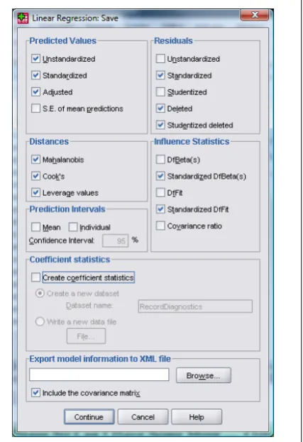
(6) C8057 (Research Methods in Psychology): Multiple Regression clears the spaces in which variables are specified. If you click on last specified, then simply click on . You can also select the tick-‐box labelled Produce all partial plots which will produce scatterplots of the residuals of the outcome variable and each of the predictors when both variables are regressed separately on the remaining predictors. Regardless of whether the previous sentence made any sense to you, these plots have several important characteristics that make them worth inspecting. First, the gradient of the regression line between the two residual variables is equivalent to the coefficient of the predictor in the regression equation. As such, any obvious outliers on a partial plot represent cases that might have undue influence on a predictor’s regression coefficient. Second, non-‐linear relationships between a predictor and the outcome variable are much more detectable using these plots. Finally, they are a useful way of detecting collinearity. For these reasons, I recommend requesting them. . and would like to return to the plot that you . Figure 5: Linear regression: plots dialog box . . There are several options for plots of the standardized residuals. First, you can select a histogram of the standardized residuals (this is extremely useful for checking the assumption of normality of errors). Second, you can ask for a normal probability plot, which also provides information about whether the residuals in the model are normally distributed. When you have selected the options you require, click on to take you back to the main regression dialog box. Saving Regression Diagnostics In this week’s lecture we met two types of regression diagnostics: those that help us assess how well our model fits our sample and those that help us detect cases that have a large influence on the model generated. In SPSS we can choose to save these diagnostic variables in the data editor (so, SPSS will calculate them and then create new columns in the data editor in which the values are placed). Click on in the main regression dialog box to activate the save new variables dialog box (see Figure 6). Once this dialog box is active, it is a simple matter to tick the boxes next to the required statistics. Most of the available options are explained in Field (2005—section 7.7.4) and Figure 6 shows, what I consider to be, a fairly basic set of diagnostic statistics. Standardized (and Studentized) versions of these diagnostics are generally easier to interpret and so I suggest selecting them in preference to the unstandardized versions. Once the regression has been run, SPSS creates a column in your data editor for each statistic requested and it has a standard set of variable names to describe each one. After the name, there will be a number that refers to the analysis that has been run. So, for the first regression run on a data set the variable names will be followed by a 1, if you carry out a second regression it will create a new set of variables with names followed by a 2 and so on. The names of the variables in the data editor are displayed below. When you have selected the diagnostics you require (by clicking in the appropriate boxes), click on to return to the main regression dialog box. . © Professor Andy Field, 2008 . . Figure 6: Dialog box for regression diagnostics . Page 6 .

(7) C8057 (Research Methods in Psychology): Multiple Regression pre_1: unstandardized predicted value; zpr_1: standardized predicted value; adj_1: adjusted predicted value; sep_1: standard error of predicted value; res_1: unstandardized residual; zre_1: standardized residual; sre_1: Studentized residual; dre_1: deleted residual; sdr_1: Studentized deleted residual; mah_1: Mahalanobis distance; coo_1: Cook’s distance; lev_1: centred leverage value; sdb0_1: standardized DFBETA (intercept); sdb1_1: standardized DFBETA (predictor 1); sdb2_1: standardized DFBETA (predictor 2); sdf_1: standardized DFFIT; cov_1: covariance ratio. . A Brief Guide to Interpretation Model Summary The model summary contains two models. Model 1 refers to the first stage in the hierarchy when only TOSCA is used as a predictor. Model 2 refers to the final model (TOSCA, and OBQ and III if they end up being included). . → In the column labelled R are the values of the multiple correlation coefficient between the predictors and the outcome. When only TOSCA is used as a predictor, this is the simple correlation between SPAI and TOSCA (0.34). 2. → The next column gives us a value of R , which is a measure of how much of the variability in the outcome is accounted for by the predictors. For the first model its value is 0.116, which means that TOSCA accounts for 11.6% of the variation in social anxiety. However, for the final model (model 2), this value increases to 0.157 or 15.7% of the variance in SPAI. Therefore, whatever variables enter the model in block 2 account for an extra (15.7-‐11.6) 4.1% of the variance in SPAI scores (this is also the value in the column labelled R-‐square change but expressed as a percentage). 2. → The adjusted R gives us some idea of how well our model generalizes and ideally we would like its value to be the 2 same, or very close to, the value of R . In this example the difference for the final model is a fair bit (0.157 – 0.143 = 0.014 or 1.4%). This shrinkage means that if the model were derived from the population rather than a sample it would account for approximately 1.4% less variance in the outcome. → Finally, if you requested the Durbin-‐Watson statistic it will be found in the last column. This statistic informs us about whether the assumption of independent errors is tenable. The closer to 2 that the value is, the better, and for these data the value is 2.084, which is so close to 2 that the assumption has almost certainly been met. ANOVA Table The next part of the output contains an analysis of variance (ANOVA) that tests whether the model is significantly better at predicting the outcome than using the mean as a ‘best guess’. Specifically, the F-‐ratio represents the ratio of the improvement in prediction that results from fitting the model (labelled ‘Regression’ in the table), relative to the inaccuracy that still exists in the model (labelled ‘Residual’ in the table). This table is again split into two sections: one for each model. If the improvement due to fitting the regression model is much greater than the inaccuracy within the model then the value of F will be greater than 1 and SPSS calculates the exact probability of obtaining the value of F by chance. For the initial model the F-‐ratio is 16.52, which is very unlikely to have happened by chance (p < .001). For the second model the value of F is 11.61, which is also highly significant (p < .001). We can interpret these results as meaning that the final model significantly improves our ability to predict the outcome variable. . © Professor Andy Field, 2008 . . Page 7 .

(8) C8057 (Research Methods in Psychology): Multiple Regression . Model Parameters The next part of the output is concerned with the parameters of the model. The first step in our hierarchy included TOSCA and although these parameters are interesting up to a point, we’re more interested in the final model because this includes all predictors that make a significant contribution to predicting social anxiety. So, we’ll look only at the lower half of the table (Model 2). . In multiple regression the model takes the form of an equation that contains a coefficient (b) for each predictor. The first part of the table gives us estimates for these b values and these values indicate the individual contribution of each predictor to the model. The b values tell us about the relationship between social anxiety and each predictor. If the value is positive we can tell that there is a positive relationship between the predictor and the outcome whereas a negative coefficient represents a negative relationship. For these data both predictors have positive b values indicating positive relationships. So, as shame (TOSCA) increases, social anxiety increases and as obsessive beliefs increase so does social anxiety; The b values also tell us to what degree each predictor affects the outcome if the effects of all other predictors are held constant. Each of these beta values has an associated standard error indicating to what extent these values would vary across different samples, and these standard errors are used to determine whether or not the b value differs significantly from zero (using the t-‐statistic that you came across last year). Therefore, if the t-‐test associated with a b value is significant (if the value in the column labelled Sig. is less than 0.05) then that predictor is making a significant contribution to the model. The smaller the value of Sig. (and the larger the value of t) the greater the contribution of that predictor. For this model, Shame (TOSCA), t(125) = 3.16, p <.01, and obsessive beliefs, t(125) = 2.46, p < .05) are significant predictors of social anxiety. From the magnitude of the t-‐statistics we can see that the Shame (TOSCA) had slightly more impact than obsessive beliefs. The b values and their significance are important statistics to look at; however, the standardized versions of the b values are easier to interpret because they are not dependent on the units of measurement of the variables. The standardized beta values are provided by SPSS and they tell us the number of standard deviations that the outcome will change as a result of one standard deviation change in the predictor. The standardized beta values (β ) are all measured in standard deviation units and so are directly comparable: therefore, they provide a better insight into the ‘importance’ of a predictor in the model. The standardized beta values for Shame (TOSCA) is 0.273, and for obsessive beliefs is 0.213. This tells us that shame has slightly more impact in the model. Excluded Variables At each stage of a regression analysis SPSS provides a summary of any variables that have not yet been entered into the model. In a hierarchical model, this summary has details of the variables that have been specified to be entered in . © Professor Andy Field, 2008 . . Page 8 .

(9) C8057 (Research Methods in Psychology): Multiple Regression subsequent steps, and in stepwise regression this table contains summaries of the variables that SPSS is considering entering into the model. The summary gives an estimate of each predictor’s b value if it was entered into the equation at this point and calculates a t-‐test for this value. In a stepwise regression, SPSS should enter the predictor with the highest t-‐statistic and will continue entering predictors until there are none left with t-‐statistics that have significance values less than 0.05. Therefore, the final model might not include all of the variables you asked SPSS to enter! In this case it tells us that if the interpretation of intrusions (III) is entered into the model it would not have a significant impact on the model’s ability to predict social anxiety, t = –0.049, p > .05. In fact the significance of this variable is almost 1 indicating it would have virtually no impact whatsoever (note also that its beta value is extremely close to zero!). . Assumptions If you want to go beyond this basic analysis, you should also look at how reliable your model is. You’ll be given a lecture about this, and Field (2009) goes through the main points in painful detail. . Writing Up Multiple Regression Analysis If you follow the American Psychological Association guidelines for reporting multiple regression then the implication seems to be that tabulated results are the way forward. They also seem in favour of reporting, as a bare minimum, the 2 standardized betas, their significance value and some general statistics about the model (such as the R ). If you do decide to do a table then the beta values and their standard errors are also very useful and personally I’d like to see the constant as well because then readers of your work can construct the full regression model if they need to. Also, if you’ve done a hierarchical regression you should report these values at each stage of the hierarchy. So, basically, you want to reproduce the table labelled coefficients from the SPSS output and omit some of the non-‐essential information. For the example in this handout we might produce a table like this: . . b . Step 1 . . . . . Constant . –54.37 . 28.62 . . . Shame (TOSCA) . 27.45 . 6.75 . .34*** . . . . Step 2 . 2 . β . SE b . . Constant . –51.49 . 28.09 . . . Shame (TOSCA) . 22.05 . 6.98 . .27** . . OCD (OBQ) . 6.92 . 2.82 . .21* . 2 . Note. R = .12 for Step 1: ∆R = .04 for Step 2 (ps < .05). * p < .05, ** p < .01, *** p < .001. . See if you can look back through the SPSS output in this handout and work out from where the values came. Things to note are: . © Professor Andy Field, 2008 . . Page 9 .

(10) C8057 (Research Methods in Psychology): Multiple Regression (1) I’ve rounded off to 2 decimal places throughout; (2) For the standardized betas there is no zero before the decimal point (because these values cannot exceed 1) but for all other values less then one the zero is present; (3) The significance of the variable is denoted by asterisks with a footnote to indicate the significance level being used (such as *p < .05, **p < .01, and ***p < .001); 2. 2. 2. (4) The R for the initial model and the change in R (denoted as ∆R ) for each subsequent step of the model are reported below the table. . Task 2 A fashion student was interested in factors that predicted the salaries of catwalk models. She collected data from 231 models. For each model she asked them their salary per day on days when they were working (salary), their age (age), how many years they had worked as a model (years), and then got a panel of experts from modelling agencies to rate the attractiveness of each model as a percentage with 100% being perfectly attractive (beauty). The data are in the file Supermodel.sav on the course website. Conduct a multiple regression to see which factor predict a model’s 3 salary? . How much variance does the final model explain? Your Answers: . . Which variables significantly predict salary? . Your Answers: . Fill in the values for the following APA format table of the results: . . b . β . SE b . . . . . Constant . . . . Age . . . . Years as a Model . . . . Attractiveness . . . . 2 . Note. R = * p < .01, ** p < .001. Write out the regression equation for the final model. 3. Answers to this task are on the CD-‐ROM of Field (2005) in the file called Answers (Chapter 5).pdf. . . © Professor Andy Field, 2008 . . Page 10 .

(11) C8057 (Research Methods in Psychology): Multiple Regression . Your Answers: . . Your Answers: . . Your Answers: . . Are the residuals as you would expect for a good model? . . Is there evidence of normality of errors, homoscedasticity and no multicollinearity? . . Task 3 Complete the multiple choice questions for Chapter 7 on the companion website to Field (2009): http://www.uk.sagepub.com/field3e/MCQ.htm. If you get any wrong, re-‐read this handout (or Field, 2009, Chapter 7) and do them again until you get them all correct. . Task 4 (Optional for Extra Practice) Go back to the output for last week’s task (does listening to heavy metal predict suicide risk). Is the model valid (i.e. are all of the assumptions met?)? This handout contains material from: . Field, A. P. (2009). Discovering statistics using SPSS: and sex and drugs and rock ‘n’ roll (3rd Edition). London: Sage. This material is copyright Andy Field (2000, 2005, 2009). . © Professor Andy Field, 2008 . . Page 11 .

(12)

No results found