472
Chapter
O
ne mathematical constant crucial to the analysis of the world is p. Thep-seriesp 6
2 1
2 1 2
3 1 2
4 1 2
5 1
2 …
approximates the value of p.The error, or remain-der, of such an approximation is the difference between the actual sum and the nth partial sum. For this p-series, the remainder is estimated by Rn 1
n.Shown here is a close-up of a high speed mi-croprocessor chip. If a computer adds 1,000,000 terms of the p-series in one second, how many places of accuracy will it achieve in 24 hours? Section 9.5 provides a discussion of p-series.
Infinite Series
Chapter 9 Overview
One consequence of the early and dramatic successes that scientists enjoyed when using calculus to explain natural phenomena was that there suddenly seemed to be no limits, so to speak, on how infinite processes might be exploited. There was still considerable mys-tery about “infinite sums” and “division by infinitely small quantities” in the years after Newton and Leibniz, but even mathematicians normally insistent on rigorous proof were inclined to throw caution to the wind while things were working. The result was a century of unprecedented progress in understanding the physical universe. ( Moreover, we can note happily in retrospect, the proofs eventually followed.)
One infinite process that had puzzled mathematicians for centuries was the summing of infinite series. Sometimes an infinite series of terms added to a number, as in
1
2 1 4
1 8 1
1
6 …1.
(You can see this by adding the areas in the “infinitely halved” unit square at the right.) But sometimes the infinite sum was infinite, as in
1
1 1 2
1 3
1 4
1
5 …
(although this is far from obvious), and sometimes the infinite sum was impossible to pin down, as in
111111…
( Is it 0? Is it 1? Is it neither?).
Nonetheless, mathematicians like Gauss and Euler successfully used infinite series to derive previously inaccessible results. Laplace used infinite series to prove the stability of the solar system (although that does not stop some people from worrying about it today when they feel that “too many” planets have swung to the same side of the sun). It was years later that care-ful analysts like Cauchy developed the theoretical foundation for series computations, send-ing many mathematicians (includsend-ing Laplace) back to their desks to verify their results.
Our approach in this chapter will be to discover the calculus of infinite series as the pio-neers of calculus did: proceeding intuitively, accepting what works and rejecting what does not. Toward the end of the chapter we will return to the crucial question of convergence and take a careful look at it.
Power Series
Geometric Series
The first thing to get straight about an infinite series is that it is not simply an example of addition. Addition of real numbers is a binaryoperation, meaning that we really add num-bers two at a time. The only reason that 123 makes sense as “addition” is that we can groupthe numbers and then add them two at a time. The associative property of addi-tion guarantees that we get the same sum no matter how we group them:
123156 and 123336.
In short, a finite sum of real numbers always produces a real number (the result of a finite number of binary additions), but an infinite sum of real numbers is something else entirely. That is why we need the following definition.
9.1
What you’ll learn about
• Geometric Series
• Representing Functions by Series
• Differentiation and Integration
• Identifying a Series
. . . and why
Power series are important in un-derstanding the physical universe and can be used to represent functions.
1/2
1/4 1/8
The partial sumsof the series form a sequence
s1a1
s2a1a2
s3a1a2a3
...
sn
nk1 ak
...
of real numbers, each defined as a finite sum. If the sequence of partial sums has a limit S
as n→, we say the series convergesto the sum S, and we write
a1a2a3…an…
k1 akS.
Otherwise, we say the series diverges.
EXAMPLE 1 Identifying a Divergent Series
Does the series 111111… converge?
SOLUTION
You might be tempted to pair the terms as
111111… .
That strategy, however, requires an infinite number of pairings, so it cannot be justified by the associative property of addition. This is an infinite series, not a finite sum, so if it has a sum it has to be the limit of its sequence of partial sums,
1, 0, 1, 0, 1, 0, 1, … .
Since this sequence has no limit, the series has no sum. It diverges.
Now try Exercise 7.
EXAMPLE 2 Identifying a Convergent Series
Does the series
130 1300 10300 … 1
3 0n … converge?
SOLUTION
Here is the sequence of partial sums, written in decimal form. 0.3, 0.33, 0.333, 0.3333, …
This sequence has a limit 0.3J, which we recognize as the fraction 1
3. The seriescon-verges to the sum 1
3. Now try Exercise 9.DEFINITION Infinite Series
An infinite seriesis an expression of the form
a1a2a3…an… , or
k1 ak.
There is an easy way to identify some divergent series. In Exercise 62 you are asked to show that whenever an infinite series
k1akconverges, the limit of the nth term as n→ must be zero.This means that if limk→ak 0 the series must diverge.
The series in Example 2 is a geometric seriesbecause each term is obtained from its preceding term by multiplying by the same number r— in this case,r1
10. ( The series of areas for the infinitely-halved square at the beginning of this chapter is also geometric.) The convergence of geometric series is one of the few infinite processes with which math-ematicians were reasonably comfortable prior to calculus. You may have already seen the following result in a previous course.This completely settles the issue for geometric series. We know which ones converge and which ones diverge, and for the convergent ones we know what the sums must be. The inter-val 1r1 is the interval of convergence.
EXAMPLE 3 Analyzing Geometric Series
Tell whether each series converges or diverges. If it converges, give its sum.
(a)
n1 3
(
12
)
n1(b) 1 1 2
1 4
1
8 …
(
1 2
)
n1
…
(c)
k0
(
35
)
k
(d) p
2
p
4 2
p83 …
SOLUTION
(a) First term is a3 and r1
2. The series converges to131
2 6.
(b)First term is a1 and r 1
2. The series converges to
1
1
1
2 23. continued
If the infinite series
k1aka1a2…ak… converges, then limk→ak0.The geometric series
aarar2ar3…arn1…
n1arn1
(c)First term is a3
501 and r35. The series converges to11 3
5 52.
(d)In this series, rp
21. The series diverges. Now try Exercises 11 and 19.We have hardly begun our study of infinite series, but knowing everything there is to know about the convergence and divergence of an entire classof series (geometric) is an impressive start. Like the Renaissance mathematicians, we are ready to explore where this might lead. We are ready to bring in x.
Representing Functions by Series
Ifx1, then the geometric series formula assures us that
1xx2x3…xn… 1
1
x
.
Consider this statement for a moment. The expression on the right defines a function whose domain is the set of all numbers x 1. The expression on the left defines a func-tion whose domain is the interval of convergence,x1. The equality is understood to hold only on this latter domain, where both sides of the equation are defined. On this domain, the series representsthe function 1
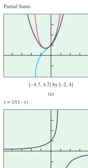
1x.The partial sums of the infinite series on the left are all polynomials, so we can graph them ( Figure 9.1). As expected, we see that the convergence is strong in the interval 1, 1but breaks down whenx1.
[image:5.684.41.191.54.340.2]The expression
n0xnis like a polynomial in that it is a sum of coefficients times powers of x, but polynomials have finite degrees and do not suffer from divergence for the wrong values of x.Just as an infinite series of numbers is not a mere sum, this series of powers of xis not a mere polynomial.[– 4.7, 4.7] by [–2, 4]
(a) Partial Sums
[– 4.7, 4.7] by [–2, 4]
(b) y = 1/(1–x)
Figure 9.1 (a) Partial sums converging to 11xon the interval (0, 1). The partial sums graphed here are 1xx2, 1
xx2x3, and 1xx2x3x4.
(b) Notice how the graphs in (a) resemble the graph of 11x on the interval 1, 1but are not even close whenx1.
The geometric series
n0xn1xx2…xn…is a power series centered at x 0. It converges on the interval 1x1, also centered at x 0. This is typical behavior, as we will see in Section 9.4. A power series either con-verges for all x, converges on a finite interval with the same center as the series, or con-verges only at the center itself.
When we setx 0 in the expression
n0cnxn c0c1xc2x2…c
nxn… ,
we get c0on the right but c0 •00on the
left. Since 00is not a number, this is a
slight flaw in the notation, which we agree to overlook. The same situation arises when we set
xa in
n0
cn(xa)n.
In either case, we agree that the expres-sion will equal c0. (It really shouldequal c0, so we are not compromising the
mathematics; we are clarifying the nota-tion we use to convey the mathematics.)
DEFINITION Power Series
An expression of the form
n0cnxnc0c1xc2x2…cnxn… is a power series centered at x0. An expression of the form n0cnxancDifferentiation and Integration
So far we have only represented functions by power series that happen to be geometric. The partial sums that converge to those power series, however, are polynomials,and we can apply calculus to polynomials. It would seem logical that the calculus of polynomials (the first rules we encountered in Chapter 3) would also apply to power series.
EXAMPLE 4 Finding a Power Series by Differentiation
Given that 1
1x is represented by the power series 1xx2…xn…on the interval 1, 1, find a power series to represent 1
1x2.SOLUTION
Notice that 1
1x2 is the derivative of 11x. To find the power series, we dif-ferentiate both sides of the equation
1 1
x 1xx
2x3…xn… .
d d
x
(
1 1
x
)
d d
x
1xx2x3…xn…
1 1
x2 12x3x24x3…nx
n1…
Finding Power Series for Other Functions
Given that 1
1x is represented by the power series 1xx2…xn…on the interval 1, 1,
1. find a power series that represents 1
1x on 1, 1.2. find a power series that represents x
1x on 1, 1.3. find a power series that represents 1
12x on 12, 12).4. find a power series that represents
1x 11x1
on 0, 2.
Could you have found the intervals of convergence yourself ?
5. Find a power series that represents
31 x 13•
(
1 1
x1
)
and give its interval of convergence.EXPLORATION 1
We have seen that the power series
n0xn represents the function 11x on the domain 1, 1. Can we find power series to represent other functions?What about the interval of convergence? Since the original series converges for 1
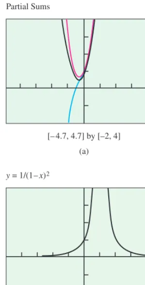
x1, it would seem that the differentiated series ought to converge on the same open interval. Graphs ( Figure 9.2) of the partial sums 12x3x2, 12x3x24x3, and 12x3x24x35x4 suggest that this is the case (although such empirical evidence does not constitute a proof). Now try Exercise 27.
The basic theorem about differentiating power series is the following.
THEOREM 1 Term-by-Term Differentiation
If fx
n0cnxanc
0c1xac2xa2…cnxan… converges for xaR, then the series
n1ncnxan1c12c2xa3c3xa2…ncnxan1… , obtained by differentiating the series forfterm by term, converges for xaR
[image:7.684.41.191.57.350.2]and representsfxon that interval. If the series forfconverges for all x, then so does the series forf.
[– 4.7, 4.7] by [–2, 4]
(a) Partial Sums
[– 4.7, 4.7] by [–2, 4]
(b) y = 1/(1–x)2
Figure 9.2 (a) The polynomial partial sums of the power series we derived for (b) 11x2seem to converge on the
open interval 1, 1. ( Example 4)
continued
Theorem 1 says that if a power series is differentiated term by term, the new series will converge on the same interval to the derivative of the function represented by the original series. This gives a way to generate new connections between functions and series.
Another way to reveal new connections between functions and series is by integration.
EXAMPLE 5 Finding a Power Series by Integration
Given that
1 1
x 1xx
2x3…xn… , 1x1 ( Exploration 1, part 1), find a power series to represent ln1x.
SOLUTION
Recall that 1
1x is the derivative of ln1x. We can therefore integrate the series for 11x to obtain a series for ln1x(no absolute value bars are neces-sary because 1x is positive for 1x1).11 x 1xx2x3…xn…
1xx2x3…1nxn…
x0
11t dt
x0
1tt2t3…1ntn…dt
ln1t
]
x0
[
t t2 2
t3 3 t44 …1n n
tn
1
1 …
]
x
0
ln1xx x
2 2
x3 3 x44 …1n n
x
n1
1 …
THEOREM 2 Term-by-Term Integration
Iffx
n0cnxanc
0c1xac2xa2…cnxan… converges for xaR, then the series
n0cn xn
a
1 n1
c0xac1x
2
a2
c2x
3
a3
…c
n
x n
a
1 n1
… ,
obtained by integrating the series forf term by term, converges for xaR
and represents
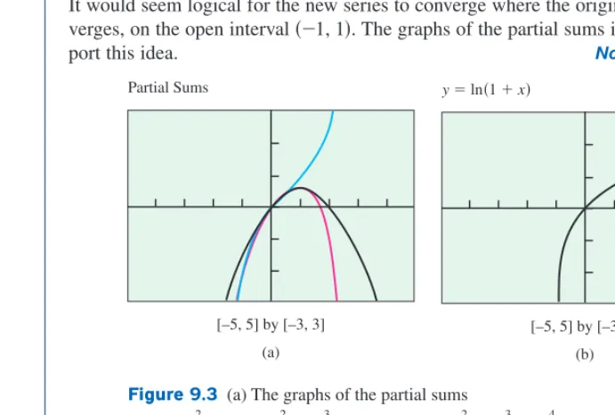
axftdt on that interval. If the series forfconverges for all x, then so does the series for the integral.It would seem logical for the new series to converge where the original series con-verges, on the open interval 1, 1. The graphs of the partial sums in Figure 9.3
sup-port this idea. Now try Exercise 33.
[–5, 5] by [–3, 3]
(a) Partial Sums
[–5, 5] by [–3, 3]
[image:8.684.210.556.60.293.2](b) y ln1 x
Figure 9.3 (a) The graphs of the partial sums
x x
2
2
, x x
2
2
x33, and x x
2
2
x3 3 x44
closing in on (b) the graph of ln1xover the interval 1, 1. ( Example 5)
Some calculators have a sequence modethat enables you to generate a sequence of partial sums, but you can also do it with simple commands on the home screen. Try entering the two multiple-step commands shown on the first screen below.
If you are successful, then every time you hit ENTER, the calculator will dis-play the next partial sum of the series
1 1 2
1 3
1 4
… n
1 1
n
….
The second screen shows the result of about 80 ENTERs. The sequence certainly seems to be converging to ln 20.6931471806….
.6997694067 .686611512 .699598525 .6867780122 .69943624 .68693624 .699281919
0 N: 1 T
N+1 N: T+(–1)^N/(
N+1) T
1
.5
The idea that the integrated series in Example 5 converges to ln1 x for all x
between 1 and 1 is confirmed by the following theorem.
Theorem 2 says that if a power series is integrated term by term, the new series will con-verge on the same interval to the integral of the function represented by the original series.
There is still more to be learned from Example 5. The original equation
1 1
x 1xx
2x3…xn…
clearly diverges at x1 (see Example 1). The behavior is not so apparent, however, for the new equation
ln1xx x
2 2
x3 3 x44 …1n n
x
n1
If we letx1 on both sides of the previous equation, we get
ln 21 1 2
1 3
1
4 … n
1 1 n
… ,
which looks like a reasonable statement. It looks even more reasonable if you look at the partial sums of the series and watch them converge toward ln 2 (see margin note). It would appear that our new series converges at 1 despite the fact that we obtained it from a series that did not! This is all the more reason to take a careful look at convergence later. Meanwhile, we can enjoy the observation that we have created a series that apparently works better than we might have expected and better than Theorem 2 could guarantee.
Finding a Power Series for tan1x
1. Find a power series that represents 1
1x2 on 1, 1.2. Use the technique of Example 5 to find a power series that represents tan1x on 1, 1.
3. Graph the first four partial sums. Do the graphs suggest convergence on the open interval 1, 1?
4. Do you think that the series for tan1x converges at x1? Can you support your answer with evidence?
EXPLORATION 2
A Series with a Curious Property
Define a functionf by a power series as follows:
fx1x x
2! 2
x
3! 3
x
4 4
! … n
xn ! … .
1. Find fx.
2. Find f0.
3. What well-known function do you supposefis?
4. Use your responses to parts 1 and 2 to set up an initial value problem that the functionfmust solve. You will need a differential equation and an initial condition.
5. Solve the initial value problem to prove your conjecture in part 3.
6. Graph the first three partial sums. What appears to be the interval of convergence?
7. Graph the next three partial sums. Did you underestimate the interval of convergence?
EXPLORATION 3
Identifying a Series
So far we have been finding power series to represent functions. Let us now try to find the function that a given power series represents.
In Exercises 1 and 2, find the first four terms and the 30th term of the sequence
{un}n1{u1,u2, … ,un, …}.
1. un n
4 2
4/3, 1, 4/5, 2/3, 1/8 2. un n
1n
In Exercises 3 and 4, the sequences are geometric an1anr, a constant). Find
(a)the common ratio r. (b)the tenth term.
(c)a rule for the nth term.
3. {2, 6, 18, 54, …} 4. {8,4, 2,1, …}
In Exercises 5–10,
(a)graph the sequence {an}.
(b)determine lim n→an.
5. an 1
n
2
n
(b) 0 6. an
(
1 1n
)
n
(b) e
7. an1n 8. a
n 1 1 2 2 n n
(b) 1
9. an2 1
n (b) 2 10. an
lnn n
1 (b) 0
Quick Review 9.1
(For help,go to Section 8.1.)Section 9.1 Exercises
1. Replace the * with an expression that will generate the series
1 1 4
1 9 1
1 6 … .
(a)
n1
1n1
(
1*
)
* n2 (b)
n01n
(
1 *)
(c)
n*
1n
(
n
1 22
)
* 32. Write an expression for the nth term,an.
(a)
n0
an1 1 3
1 9 2
1 7
811 …
1 3n
(b)
n1
an1 1 2 1 3 1 4 1 5
… (1
n
)n1
(c)
n0
an50.50.050.0050.0005… 1 5 0n
In Exercises 3–6, tell whether the series is the same as
n1(
12)
n1.
3.
n1
(
12)
n1Different 4.
n0
(
12
)
nSame
5.
n0
1n
(
1 2)
n
Same 6.
n1
2n 1
1
n
Different
In Exercises 7–10, compute the limit of the partial sums to determine whether the series converges or diverges.
7. 11.11.111.1111.1111… Diverges
8. 211111… Diverges
9. 1
2 1 4 1 8 … 2 1 k … Converges
10.30.50.050.0050.0005… Converges
In Exercises 11–20, tell whether the series converges or diverges. If it converges, give its sum.
11. 1 2
3
(
2 3)
2
(
23)
3
…
(
2 3)
n
… Converges; sum 3
12.12345…1nn1… Diverges
13.
n0
(
54
)(
23)
n14.
n0
(
23
)(
54)
nDiverges
15.
n0
cosnp Diverges
16.30.30.030.0030.0003…30.1n…
17.
n0
sinn
(
p4 np
)
Converges; sum 2 218.1
2 2 3 3 4 4 5 … n n 1 … Diverges 19.
n1
(
pe
)
n20.
n0
65n n
1
Converges; sum 1
In Exercises 21–24, find the interval of convergence and the function of xrepresented by the geometric series.
21.
n0
2nxn 22.
n01nx1n23.
n0
(
12
)
nx3n 24.
n03(
x 2 1)
n
In Exercises 25 and 26, find the values of xfor which the geometric series converges and find the function of xit represents.
25.
n0
sinnx 26.
n0tannxIn Exercises 27–30, use the series and the function f(x) that it represents from the indicated exercise to find a power series for f(x).
27.Exercise 21 28. Exercise 22
29.Exercise 23 30. Exercise 24 1, 1/2,1/3, 1/4, 1/30
(a)3 (b)39,366 (c)an2(3n1) (a)1/2 (b)1/64
(c) an8(1/2)n1 8(0.5)n1
(b) The limit does not exist.
* (n1)2
Converges; sum 15/4
Converges; sum 30/11
In Exercises 31–34, use the series and the function f(x) that it represents from the indicated exercise to find a power series for
x0f(t) dt.
31. Exercise 21 32.Exercise 22
33. Exercise 23 34.Exercise 24
35. Writing to Learn Each of the following series diverges in a slightly different way. Explain what is happening to the sequence of partial sums in each case.
(a)
n1
2n (b)
n0
1n (c)
n11n2n
36.Prove that
n0penn
p
e
diverges.
37.Solve for x:
n0
xn 20. x 19/20
38.Writing to Learn Explain how it is possible, given any real number at all, to construct an infinite series of non-zero terms that converges to it.
39.Make up a geometric series arn1 that converges to the
number 5 if
(a) a 2 (b) a 132
In Exercises 40 and 41, express the repeating decimal as a geometric series and find its sum.
40. 0.21J 41. 0.234J
In Exercises 42–47, express the number as the ratio of two integers.
42. 0.7J0.7777… 7/9
43.0.dJ0.dddd… , where dis a digit d/9
44.0.06J0.06666… 1/15 45. 1.414J1.414 414 414…
46.1.24123J1.24 123 123 123… 41,333/33,300
47.3.1J42857JJ3.142857 142857… 22/7
48.Bouncing Ball A ball is dropped from a height of 4 m. Each time it strikes the pavement after falling from a height of hm, it rebounds to a height of 0.6hm. Find the total distance the ball travels up and down. 16 meters
49.(Continuation of Exercise 48) Find the total number of seconds that the ball in Exercise 48 travels. (Hint:A freely falling ball travels 4.9t2meters in tseconds, so it will fall h
meters in h4.9 seconds. Bouncing from ground to apex takes the same time as falling from apex to ground.)
50. Summing Areas The figure below shows the first five of an infinite sequence of squares. The outermost square has an area of 4 m2. Each of the other squares is obtained by joining
the midpoints of the sides of the preceding square. Find the sum of the areas of all the squares. 8 m2
51.Summing Areas The accompanying figure shows the first three rows and part of the fourth row of a sequence of rows of semicircles. There are 2nsemicircles in the nth row, each of radius 12n. Find the sum of the areas of all the semicircles.
52.Sum of a Finite Geometric Progression Let aand rbe real numbers with r 1, and let
Saarar2ar3…arn1.
(a) Find SrS. SrSaarn
(b) Use the result in part (a) to show that S a
1
a r rn .
53. Sum of a Convergent Geometric Series Exercise 52 gives a formula for the nth partial sum of an infinite geometric series. Use this formula to show that n1arn1 diverges when
r1 and converges to a1r when r1.
In Exercises 54–59, find a power series to represent the given function and identify its interval of convergence. When writing the power series, include a formula for the nth term.
54.
1 1
3x
55.
1
x
2x
56.
1 3
x3
57.
1 1
x4
58.
4 1
x
14
(
11x1)
59.2 1
x
(Hint:Rewrite 2x.) 1/2
1/4 1/8
(a)
n1
2
3 5n1
(b)
n1
123
130n1
157/111
7.113 seconds
2
60.Find the value of bfor which 1ebe2be3b…9.
61.Let Sbe the series
n0(
1tt
)
n, t 0.
(a) Find the value to which Sconverges when t1. 2
(b) Determine all values of tfor which Sconverges. t 1/2
(c) Find all values of tthat make the sum of Sgreater than 10.
62.nth Term Test Assume that the series k1akconverges to S.
(a) Writing to Learn Explain why limn→kk1nak S.
(b)Show that SnSn1an, where Sndenotes the nth partial sum of the series.
(c) Show that limn→an 0.
63.A Series for ln x Starting with the power series found for 1x
in Exploration 1, Part 4, find a power series for lnx centered at x1.
64. Differentiation Use differentiation to find a series for
fx21x3. What is the interval of convergence of
your series?
65. Group Activity Intervals of Convergence How much can the interval of convergence of a power series be changed by integration or differentiation? To be specific, suppose that the power series
fxc0c1xc2x2…c nxn…
converges for 1x1 and diverges for all other values of x.
(a) Writing to Learn Could the series obtained by integrating the series forfterm by term possibly converge for 2x2? Explain. (Hint:Apply Theorem 1, not Theorem 2.)
(b)Writing to Learn Could the series obtained by differentiating the series forfterm by term possibly converge for 2x2? Explain.
Standardized Test Questions
You should solve the following problems without using a graphing calculator.
66.True or False The series 1 2 1. 2 01 (1.0 2 1)2 … (1.0 2 1)n …
converges. Justify your answer.
67. True or False The series 1 1 2
1 4
1 8 1
1 6 … diverges. Justify your answer.
68.Multiple Choice To which of the following numbers does the series 1 1
3 1 9 2
1
7 …converge? C
(A) 23 (B) 98 (C) 32 (D) 2 (E) It diverges
In Exercises 69–71, use the geometric series n0(x1)n, which represents the function f(x).
69.Multiple Choice Find the values of xfor which the series converges. A
(A) 0x2 (B) 0x1 (C) 1x0
(D)1x1 (E) 2x0
70.Multiple Choice Which of the following is the function that the power series represents? E
(A) x 1 1 (B) 1 1 2x
(C) 1
x (D) x
1 2 (E) 2 1 x
71.Multiple Choice Which of the following is a function that
x0f(t) dtrepresents? D
(A) ln
x 2 2 (B) ln x 2 2 (C) (x 1 2)2(D) ln
x 22
(E) ln x 22
Exploration
72.Let ft
1 4
t2
and Gx
x
0
ftdt.
(a) Find the first four nonzero terms and the general term for a power series for ft centered at t0.
(b) Find the first four nonzero terms and the general term for a power series for Gx centered at x0.
(c) Find the interval of convergence of the power series in part (a).
(d) The interval of convergence of the power series in part (b) is almost the same as the interval in part (c), but includes two more numbers. What are the numbers?
Extending the Ideas
The sequence {an} converges to the number Lif to every positive number ethere corresponds an integer Nsuch that for all n,
nN ⇒ anLe.
Lis the limit of the sequence and we write limn→anL. If no such number Lexists, we say that {an} diverges.
73. Tail of a Sequence Prove that if {an} is a convergent sequence, then to every positive number ethere corresponds an integer Nsuch that for all mand n,
mN and nN ⇒ amane.
(Hint:Let limn→anL. As the terms approach L, how far apart can they be?)
74. Uniqueness of Limits Prove that limits of sequences are unique. That is, show that if L1and L2are numbers such that limn→anL1 and limn→anL2, then L1L2.
75.Limits and Subsequences Prove that if two subsequences of a sequence {an} have different limits L1 L2, then {an} diverges.
76. Limits and Asymptotes
(a)Show that the sequence with nth term an3n1n1 converges.
(b)If limn→anL, explain why yL is a horizontal asymptote of the graph of the function
fx 3 x x
1 1
obtained by replacing nby xin the nth term.
bln(8/9)
t9
x (x
2 1)2
(x3 1)3 (1)n1n (x1)n Interval:1x1
False. It diverges because it is a geometric series with ratio 1.01 that is greater than 1.
Taylor Series
Constructing a Series
A comprehensive understanding of geometric series served us well in Section 9.1, enabling us to find power series to represent certain functions, and functions that are equivalent to certain power series (all of these equivalencies being subject to the condition of convergence). In this section we learn a more general technique for constructing power series, one that makes good use of the tools of calculus.
Let us start by constructing a polynomial.
9.2
What you’ll learn about
• Constructing a Series
• Series for sin xand cos x
• Beauty Bare
• Maclaurin and Taylor Series
• Combining Taylor Series
• Table of Maclaurin Series
. . . and why
The partial sums of a Taylor se-ries are polynomials that can be used to approximate the function represented by the series.
Designing a Polynomial to Specifications
Construct a polynomial Pxa0a1xa2x2a
3x3a4x4 with the follow-ing behavior at x0:
P01,
P02,
P03,
P04, and
P405.
This task might look difficult at first, but when you try it you will find that the pre-dictability of differentiation when applied to polynomials makes it straightforward. (Be sure to check this out before you move on.)
EXPLORATION 1
There is nothing special about the number of derivatives in Exploration 1. We could have prescribed the value of the polynomial and its first nderivatives atx0 for any n
and found a polynomial of degree at most nto match. Our plan now is to use the technique of Exploration 1 to construct polynomials that approximate functions by emulating their behavior at 0.
EXAMPLE 1 Approximating ln (1x) by a Polynomial
Construct a polynomial Pxa0a1xa2x2a
3x3a4x4 that matches the behavior of ln1x at x0 through its first four derivatives. That is,
P0ln1x at x0,
P0ln1x at x0,
P0ln1x at x0,
P0ln1x at x0, and
P40ln1x4 at x0.
SOLUTION
This is just like Exploration 1, except that first we need to find out what the numbers are.
P0ln1x
|
x00
P0 1
1
x
|
x0
1
P0
1 1
x2
|
x0 1
P0 1
2
x3
|
x0
2
P40
1 6
x4
|
x0 6
In working through Exploration 1, you probably noticed that the coefficient of the term
xnin the polynomial we seek is Pn0divided by n!. The polynomial is Px0x x
2 2
x
3 3
x
4 4
.
Now try Exercise 1.
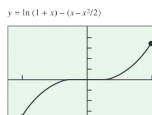
We have just constructed the fourth order Taylor polynomial for the function ln1xat x0. You might recognize it as the beginning of the power series we dis-covered for ln1xin Example 5 of Section 9.1, when we came upon it by integrat-ing a geometric series. If we keep gointegrat-ing, of course, we will gradually reconstruct that entire series one term at a time, improving the approximation near x0 with every term we add. The series is called the Taylor seriesgenerated by the function ln1x
at x0.
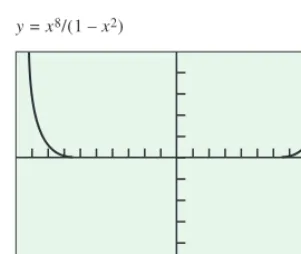
You might also recall Figure 9.3, which shows how the polynomial approximations con-verge nicely to ln1xnear x0, but then gradually peel away from the curve as xgets farther away from 0 in either direction. Given that the coefficients are totally determined by specifying behavior at x0, that is exactly what we ought to expect.
Series for sin
x
and cos
x
We can use the technique of Example 1 to construct Taylor series about x0 for any func-tion, as long as we can keep taking derivatives there. Two functions that are particularly well-suited for this treatment are the sine and cosine.
EXAMPLE 2 Constructing a Power Series for sinx
Construct the seventh order Taylor polynomial and the Taylor series for sinx
at x0.
SOLUTION
We need to evaluate sinx and its first seven derivatives at x0. Fortunately, this is not hard to do.
sin00
sin0 cos0 1 sin0 sin0 0 sin0 cos0 1 sin40 sin0 0 sin50 cos0 1
...
The pattern 0, 1, 0,1 will keep repeating forever.
The unique seventh order Taylor polynomial that matches all these derivatives at x0 is
P7x01x0x2 3
1 !
x30x4 5
1 !
x50x6 7
1 !
x7
x x
3! 3
x
5! 5
x
7! 7
.
P7 is the seventh order Taylor polynomial for sinxat x0. ( It also happens to be of seventh degree,but that does not always happen. For example, you can see that P8for sinxwill be the same polynomial as P7.)
To form the Taylor series, we just keep on going:
x x
3! 3
x
5! 5
x
7! 7
x
9! 9
…
n0
1n 2
x n 2
n
1 1
!
.
Now try Exercise 3.
Beauty Bare
Edna St. Vincent Millay, an early twentieth-century American poet, referring to the experience of simultaneously seeing and understanding the geometric underpinnings of nature, wrote “Euclid alone has looked on Beauty bare.” In case you have never experienced that sort of reverie when gazing upon something geometric, we intend to give you that opportunity now.
In Example 2 we constructed a power series for sinxby matching the behavior of sinx
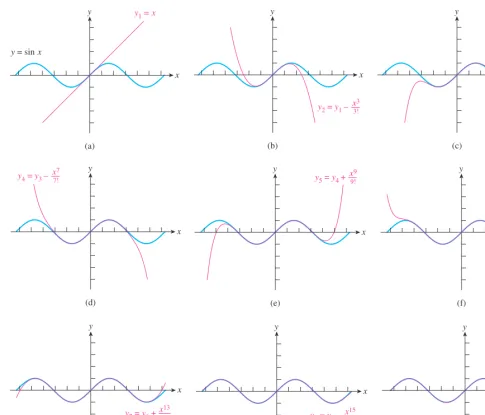
atx0. Let us graph the first nine partial sums together with ysinxto see how well we did ( Figure 9.4).
Behold what is occurring here! These polynomials were constructed to mimic the behavior of sinxnear x0. The only information we used to construct the coefficients of these polynomials was information about the sine function and its derivatives at 0. Yet, somehow, the information atx0 is producing a series whose graph not only looks like sine near the origin, but appears to be a clone of the entire sine curve. This is no deception, either; we will show in Section 9.3, Example 3 that the Taylor series for sinxdoes, in fact, converge to sinxover the entire real line. We have managed to construct an entire function by knowing its behavior at a single point! ( The same is true about the series for cosx
found in Exploration 2.)
We still must remember that convergence is an infinite process. Even the one-billionth order Taylor polynomial begins to peel away from sinxas we move away from 0, although imperceptibly at first, and eventually becomes unbounded, as any polynomial must. Nonetheless, we can approximate the sine of anynumber to whatever accuracy we want if we just have the patience to work out enough terms of this series!
This kind of dramatic convergence does not occur for all Taylor series. The Taylor poly-nomials for ln1xdo not converge outside the interval from 1 to 1, no matter how many terms we add.
A Power Series for the Cosine
Group Activity
1. Construct the sixth order Taylor polynomial and the Taylor series at x0 for cosx.
2. Compare your method for attacking part 1 with the methods of other groups. Did anyone find a shortcut?
Maclaurin and Taylor Series
If we generalize the steps we followed in constructing the coefficients of the power series in this section so far, we arrive at the following definition.
x y y1 = x
y = sin x
(a)
x y
(b)
y2 = y1 –x3 3!
x y
(c)
y3 = y2 +x5 5!
x y
(d) y4 = y3 – x7
7!
x y
(e)
y5 = y4 +x9 9!
x y
(f)
y6 = y5 –x11 11!
x y
(g)
y7 = y6 + x13 13!
x y
(h)
y8 = y7 – x15 15!
x y
(i)
[image:16.684.82.567.50.464.2]y9 = y8 + x17 17!
Figure 9.4 ysin xand its nine Taylor polynomials P1,P3, … ,P17for 2px2p. Try graphing these functions in the window 2p,2pby 5, 5.
DEFINITION Taylor Series Generated by fat x0
(Maclaurin Series)
Letfbe a function with derivatives of all orders throughout some open interval containing 0. Then the Taylor series generated byfat x0 is
f0f0x f
2 ! 0
x2… fn
n
! 0
xn…
k0
fk
k
! 0
xk.
We usef0to meanf. Everypower series constructed in this way converges to the func-tionfat x0, but we have seen that the convergence might well extend to an interval con-taining 0, or even to the entire real line. When this happens, the Taylor polynomials that form the partial sums of a Taylor series provide good approximations forfnear 0.
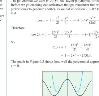
EXAMPLE 3 Approximating a Function Near 0
Find the fourth order Taylor polynomial that approximates ycos 2x near x0.
SOLUTION
The polynomial we want is P4x, the Taylor polynomial for cos 2x at x0. Before we go cranking out derivatives though, remember that we can use a known power series to generate another, as we did in Section 9.1. We know from Exploration 2 that
cosx1 x 2!
2
x4!4 …1n 2
x n 2n
! … . Therefore,
cos 2x1 2 2
x
! 2
2
4
x
! 4
…1n
2 2
x n
2
! n
… .
So,
P4x1 2 2
x
! 2
24x!4 12x22
3x4.The graph in Figure 9.5 shows how well the polynomial approximates the cosine near
x0. Now try Exercise 5.
Who invented Taylor series?
Brook Taylor (1685 –1731) did not invent Taylor series, and Maclaurin series were not developed by Colin Maclaurin (1698 –1746). James Gregory was al-ready working with Taylor series when Taylor was only a few years old, and he published the Maclaurin series for tanx, secx,arctanx,and arcsecxten years before Maclaurin was born. Nicolaus Mer-cator discovered the Maclaurin series for ln1 xat about the same time.
Taylor was unaware of Gregory’s work when he published his book Methodus In-crementorum Directa et Inversain 1715, containing what we now call Taylor se-ries. Maclaurin quoted Taylor’s work in a calculus book he wrote in 1742. The book popularized series representations of functions and although Maclaurin never claimed to have discovered them, Taylor series centered atx 0 became known as Maclaurin series. History evened things up in the end. Maclaurin, a brilliant mathematician, was the original discov-erer of the rule for solving systems of equations that we call Cramer’s rule.
[image:17.684.200.520.301.613.2][–3, 3] by [–2, 2]
Figure 9.5 The graphs of y12x223x4and ycos 2x
near x0. ( Example 3)
These polynomial approximations can be useful in a variety of ways. For one thing, it is easy to do calculus with polynomials. For another thing, polynomials are built using only the two basic operations of addition and multiplication, so computers can handle them easily.
The partial sum
Pnx
nk0
fk
k
! 0
xk
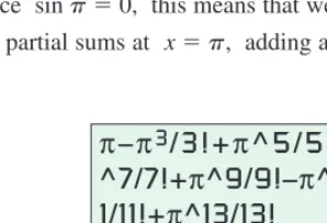
Approximating sin 13
How many terms of the series
n01n 2x n 2
n
1 1
!
are required to approximate sin 13 accurate to the third decimal place?
1. Find sin 13 on your calculator ( radians, of course).
2. Enter these two multiple-step commands on your home screen. They will give you the first order and second order Taylor polynomial approximations for sin 13. Notice that the second order approximation, in particular, is not very good.
3. Continue to hit ENTER. Each time you will add one more term to the Taylor polynomial approximation. Be patient; things will get worse before they get better.
4. How many terms are required before the polynomial approximations stabilize in the thousandths place for x13?
EXPLORATION 3
0 N: 13 T
N+1 N: T+(–1)^N*1
3^(2N+1)/(2N+1)!
T
13
–353.1666667
This strategy for approximation would be of limited practical value if we were restricted to power series atx0 — but we are not. We can match a power series withfin the same way at any value xa, provided we can take the derivatives. In fact, we can get a formula for doing that by simply “shifting horizontally” the formula we already have.
DEFINITION Taylor Series Generated by fat xa
Letfbe a function with derivatives of all orders throughout some open interval containing a.Then the Taylor series generated byfat xais
fafaxa f
2 !
a
xa2… fn
n
!
a
xan…
k0
fkk!axak. The partial sum
Pnx
nk0
fkk!axak
EXAMPLE 4 A Taylor Series at x2
Find the Taylor series generated by fxex at x2.
SOLUTION
We first observe that f2f2f2…fn2e2. The series, therefore, is
exe2e2x2 2
e2 !
x22…
n e2
!
x2n…
k0
(
ke2!
)
x2k.We illustrate the convergence near x2 by sketching the graphs of yexand yP3x
in Figure 9.6. Now try Exercise 13.
EXAMPLE 5 A Taylor Polynomial for a Polynomial
Find the third order Taylor polynomial for fx2x33x24x5
(a)at x0. (b)at x1. SOLUTION
(a)This is easy. This polynomial is already written in powers of xand is of degree three, so it is its own third order (and fourth order, etc.) Taylor polynomial at x0.
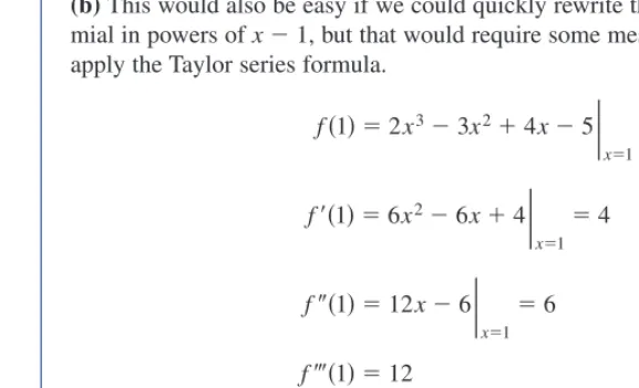
(b)This would also be easy if we could quickly rewrite the formula forfas a polyno-mial in powers of x1, but that would require some messy tinkering. Instead, we apply the Taylor series formula.
f12x33x24x5
|
x1 2f16x26x4
|
x14
f112x6
|
x16
f112 So,
P3x 24x1 2
6 !
x12 1
3 2
!
x13
2x133x124x12.
This polynomial function agrees withfat every value of x(as you can verify by multi-plying it out) but it is written in powers of x1instead of x. Now try Exercise 15.
Combining Taylor Series
[image:19.684.203.492.385.560.2]On the intersection of their intervals of convergence, Taylor series can be added, sub-tracted, and multiplied by constants and powers of x, and the results are once again Taylor series. The Taylor series forfxgxis the sum of the Taylor series for fxand the [–1, 4] by [–10, 50]
Figure 9.6 The graphs of yexand
Taylor series for gxbecause the nth derivative offgisfngn, and so on. We can obtain the Maclaurin series for 1cos 2x
2 by substituting 2xin the Maclaurin series for cos x, adding 1, and dividing the result by 2. The Maclaurin series for sinxcosxis the term -by-term sum of the series for sinxand cosx.We obtain the Maclaurin series for [image:20.684.216.581.235.689.2]xsinxby multiplying all the terms of the Maclaurin series for sinxby x.
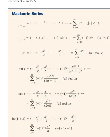
Table of Maclaurin Series
We conclude the section by listing some of the most useful Maclaurin series, all of which have been derived in one way or another in the first two sections of this chapter. The exercises will ask you to use these series as basic building blocks for constructing other series (e.g., tan1x2or 7xex). We also list the intervals of convergence, although rigorous proofs of convergence are deferred until we develop convergence tests in Sections 9.4 and 9.5.
Maclaurin Series
11 x 1xx2…xn…
n0
xn x1
1 1
x 1xx
2…xn…
n01nxn x1
ex1x x 2!
2
… x
n n
! …
n0
xnn! (all real x)
sinxx x
3! 3
x
5! 5
…1n 2
x n 2
n1
1! …
n0
1n 2
x n 2
n1
1!
(all real x)
cosx1 x 2!
2
x
4! 4
…1n 2
x n 2n
! …
n0
1n 2
x n 2n
!
(all real x)
ln1xx x
2 2
x
3 3
…1n1x n
n …
n1
1n1x n
n
1x1
tan1xx x 3
3
x
5 5
…1n 2
x n
2n
1
1 …
n0
1n 2
x n
2n
1
1
In Exercises 1–5, find a formula for the nth derivative of the function.
1. e2x 2ne2x 2.
x
1 1
(1)nn! (x 1)(n1)
3. 3x 3x(1n 3)n 4. lnx (1)n1(n 1)!xn
5. xn n!
In Exercises 6–10, find dydx.(Assume that letters other than
xrepresent constants.)
6. y x
n! n
(nxn11)! 7. y 2
nx
n
!
an
8. y1n
2n x2
n1
1!
9. y x
2n a !
2n
10.y 1
n!
xn
Quick Review 9.2
(For help, go to Sections 3.3 and 3.6.)Section 9.2 Exercises
In Exercises 1 and 2, construct the fourth order Taylor polynomial at
x0 for the function.
1. f(x)1x2 2. f(x)e2x
In Exercises 3 and 4, construct the fifth order Taylor polynomial and the Taylor series for the function at x0.
3. f(x)
x
1 2
4. f(x)e1x
In Exercises 5–12, use the table of Maclaurin series on the preceding page. Construct the first three nonzero terms and the general term of the Maclaurin series generated by the function and give the interval of convergence.
5. sin 2x 6. ln1x
7. tan1x2 8. 7x ex
9. cosx2(Hint:cos x2cos 2cos xsin 2sin x
10.x2cosx 11.
1
x x3
12.e2x
In Exercises 13 and 14, find the Taylor series generated by the function at the given point.
13. f(x)
x
1 1
, x2 14.f(x)ex2, x1
In Exercises 15–17, find the Taylor polynomial of order 3 generated byf
(a) at x0; (b)at x1.
15.fxx32x4
16.fx2x3x23x8
17.fxx4
In Exercises 18–21, find the Taylor polynomials of orders 0, 1, 2, and 3 generated byfat xa.
18. fx 1
x, a2 19. fxsinx, ap4
20. fxcosx, ap4 21. fxx, a4
22.Letfbe a function that has derivatives of all orders for all real numbers. Assume f04, f05, f0 8, and f06.
(a) Write the third order Taylor polynomial forfat x0 and use it to approximate f0.2.
(b)Write the second order Taylor polynomial forf, the derivative off, at x0 and use it to approximate f0.2.
23.Letfbe a function that has derivatives of all orders for all real numbers. Assume f14, f1 1, f13, and f12.
(a) Write the third order Taylor polynomial forfat x1 and use it to approximate f1.2.
(b) Write the second order Taylor polynomial forf, the derivative off, at x1 and use it to approximate f1.2.
24.The Maclaurin series forfxis
fx1 2
x
! x
3!
2
x 4!
3
…
n
xn
1! … .
(a) Find f0 and f100.
(b) Let gxx fx. Write the Maclaurin series for gx, showing the first three nonzero terms and the general term.
(c) Write gxin terms of a familiar function without using series.
25. (a) Write the first three nonzero terms and the general term of the Taylor series generated by ex2 at x0.
(b) Write the first three nonzero terms and the general term of a power series to represent
gx e
x
x
1 .
(c) For the function gin part (b), find g(1) and use it to show that
n1nn1! 1.26.Let
ft
1 2
t2
and Gx
x
0
ftdt.
(a) Find the first four terms and the general term for the Maclaurin series generated byf.
(b) Find the first four nonzero terms and the Maclaurin series for G.