7.LinearProgrammimgSimplex.pdf

(1)

115 TEACHING

SUGGESTIONS

Teaching Suggestion 9.1:Meaning of Slack Variables.

Slack variables have an important physical interpretation and rep-resent a valuable commodity, such as unused labor, machine time, money, space, and so forth.

Teaching Suggestion 9.2:Initial Solutions to LP Problems. Explain that all initial solutions begin with X10, X20 (that is, the real variables set to zero), and the slacks are the variables with nonzero values. Variables with values of zero are called nonbasic and those with nonzero values are said to be basic.

Teaching Suggestion 9.3:Substitution Rates in a Simplex Tableau. Perhaps the most confusing pieces of information to interpret in a simplex tableau are “substitution rates.” These numbers should be explained very clearly for the first tableau because they will have a clear physical meaning. Warn the students that in subsequent tableaus the interpretation is the same but will not be as clear be-cause we are dealing with marginalrates of substitution.

Teaching Suggestion 9.4:Hand Calculations in a Simplex Tableau.

It is almost impossible to walk through even a small simplex prob-lem (two variables, two constraints) without making at least one arithmetic error. This can be maddening for students who know what the correct solution should be but can’t reach it. We suggest two tips:

1. Encourage students to also solve the assigned problem by computer and to request the detailed simplex output. They can now check their work at each iteration. 2. Stress the importance of interpreting the numbers in the

tableau at each iteration. The 0s and 1s in the columns of the variables in the solutions are arithmetic checks and balances at each step.

Teaching Suggestion 9.5:Infeasibility Is a Major Problem in Large LP Problems.

As we noted in Teaching Suggestion 7.6, students should be aware that infeasibility commonly arises in large, real-world-sized prob-lems. This chapter deals with how to spot the problem (and is very straightforward), but the real issue is how to correct the improper formulation. This is often a management issue.

ALTERNATIVE

EXAMPLES

Alternative Example 9.1: Simplex Solution to Alternative Ex-ample 7.1 (see Chapter 7 of Solutions Manual for formulation and graphical solution).

This is not an optimum solution since the X1column contains a positive value. More profit remains ($C\vper #1).

This is an optimum solution since there are no positive values in the C_jZ_jrow. This says to make 4 of item #2 and 8 of item #1 to get a profit of $60.

Alternative Example 9.2: Set up an initial simplex tableau, given the following two constraints and objective function:

Minimize Z8X16X2 Subject to: 2X₁4X₂8

3X12X26

The constraints and objective function may be rewritten as:

Minimize 8X16X20S10S2MA1MA2 2X14X21S10S21A10A28 3X12X20S11S20A11A26

9

C H A P T E R

Linear Programming: The Simplex Method

1st Iteration

Cjl Solution 3 9 0 0

b Mix X1 X2 S1 S2 Quantity

0 S1 1 4 1 0 24

0 S2 1 2 0 1 16

Zj 0 0 0 0 0

CjZj 3 9 0 0

2nd Iteration

9 X2 1⁄4 1 1⁄4 0 6

0 S2 1⁄2 0 1⁄2 1 4

Zj 9⁄4 9 9⁄4 0 54

CjZj 3⁄4 0 9⁄4 0

3rd/Final Iteration

9 X2 0 1 1⁄2 1⁄2 4

3 X1 1 0 13⁄2 23⁄2 8

Zj 3 9 3⁄2 3⁄2 60

(2)

The first tableau would be:

The second tableau:

The third and final tableau:

Printout for Alternate Example 9-3

Cjl Solution 8 6 0 0 M M

b Mix X1 X2 S1 S2 A1 A2 Quantity

M A1 2 4 1 0 1 0 8

M A2 3 2 0 1 0 1 6

Zj 5M 6M M M M M 14M

CjZj 8 5M 6 6M M M 0 0

6 X2 1⁄2 1 1⁄4 0 1⁄4 0 2

M A2 2 0 1⁄2 1 1⁄2 1 2

Zj 3 2M 6 3⁄21⁄2M M 3⁄21⁄2M M 12 2M

CjZj 5 2M 0 3⁄21⁄2M M 3⁄23⁄2M 0

6 X2 0 1 3⁄8 1⁄4 3⁄8 1⁄4 3⁄2

8 X1 1 0 1⁄4 1⁄2 1⁄4 1⁄2 1

Zj 8 6 1⁄4 5⁄2 1⁄4 5⁄2 17

CjZj 0 0 1⁄4 5⁄2 M1⁄4 M5⁄2

Simplex Tableau : 2

\Cj 3.000 9.000 0.000 0.000

Cb\ Basis Bi x 1 x 2 s 1 s 2

9.000 x 2 4.000 0.000 1.000 0.500 0.500 3.000 x 1 8.000 1.000 0.000 1.000 2.000

Zj 60.000 3.000 9.000 1.500 1.500

Cj Zj 0.000 0.000 1.500 1.500

Final Optimal Solution

Z 60.000

Variable Value Reduced Cost

x 1 8.000 0.000

x 2 4.000 0.000

Constraint Slack/Surplus Shadow Price

C 1 0.000 1.500

C 2 0.000 1.500

Objective Coefficient Ranges

Lower Current Upper Allowable Allowable Variables Limit Values Limit Increase Decrease

x 1 2.250 3.000 4.500 1.500 0.750

x 2 6.000 9.000 12.000 3.000 3.000

Right-Hand-Side Ranges

Lower Current Upper Allowable Allowable Constraints Limit Values Limit Increase Decrease

C 1 16.000 24.000 32.000 8.000 8.000

C 2 12.000 16.000 24.000 8.000 4.000

A minimal, optimum cost of 17 can be achieved by using 1 of a type #1 and C\xof a type #2.

Alternative Example 9.3: Referring back to Hal, in Alternative Example 7.1, we had a formulation of:

Maximize Profit $3X1$9X2 Subject to: 1X14X224 clay

1X12X216 glaze where X1small vases made

X2large vases made

The optimal solution was X18, X24. Profit $60.

Using software (see the printout to the left), we can perform a variety of sensitivity analyses on this solution.

Alternative Example 9.4: Levine Micros assembles both laptop and desktop personal computers. Each laptop yields $160 in profit; each desktop $200.

The firm’s LP primal is:

Maximize profit $160X1$200X2 subject to: 1X12X220 labor hours

9X19X2108 RAM chips 12X16X2$120 royalty fees where X1no. laptops assembled daily

(3)

Here is the primal optimal solution and final simplex tableau.

or X14, X28, S3$24 in slack royalty fees paid Profit $2,240/day

Here is the dualformulation:

Minimize Z20y1108y2120y3 subject to: 1y19y212y3160 2y19y26y3200 Here is the dual optimal solution and final tableau.

This means

y1marginal value of one more labor hour $40

y2marginal value of one more RAM chip $13.33

y3marginal value of one more $1 in royalty fees $0

SOLUTIONS TO

DISCUSSION

QUESTIONS

AND

PROBLEMS

9-1. The purpose of the simplex method is to find the optimal solution to LP problems in a systematic and efficient manner. The procedures are described in detail in Section 9.6.

9-2. Differencesbetween graphical and simplex methods: (1) Graphical method can be used only when two variables are in model; simplex can handle any dimensions. (2) Graphical method must evaluate all corner points (if the corner point method is used); simplex checks a lesser number of corners. (3) Simplex method can be automated and computerized. (4) Simplex method involves use of surplus, slack, and artificial variables but provides useful economic data as a by-product.

Similarities:(1) Both methods find the optimal solution at a corner point. (2) Both methods require a feasible region and the same problem structure, that is, objective function and constraints. The graphical method is preferable when the problem has two variables and only two or three constraints (and when no com-puter is available).

9-3. Slack variables convert constraints into equalities for the simplex table. They represent a quantity of unused resource and have a zero coefficient in the objective function.

Surplus variables convert constraints into equalities and represent a resource usage above the minimum required. They, too, have a zero coefficient in the objective function.

Artificial variables have no physical meaning but are used with the constraints that are or . They carry a high coefficient, so they are quickly removed from the initial solution.

9-4. The number of basic variables (i.e., variables in the solution) is always equal to the number of constraints. So in this case there will be eight basic variables. A nonbasic variable is one that is not currently in the solution, that is, not listed in the solu-tion mix column of the tableau. It should be noted that while there will be eight basic variables, the values of some of them may be zero.

9-5. Pivot column:Select the variable column with the largest positive C_jZ_jvalue (in a maximization problem) or smallest neg-ative CjZj value (in a minimization problem).

Pivot row: Select the row with the smallest quantity-to-column ratio that is a nonnegative number.

Pivot number:Defined to be at the intersection of the pivot column and pivot row.

9-6. Maximization and minimization problems are quite similar in the application of the simplex method. Minimization problems usually include constraints necessitating artificial and surplus vari-ables. In terms of technique, the C_j Z_jrow is the main differ-ence. In maximization problems, the greatest positive CjZj indi-cates the new pivot column; in minimization problems, it’s the smallest negative CjZj. The Zjentry in the “quantity” column stands for profit contribution or cost, in maximization and mini-mization problems, respectively.

9-7. The Zjvalues indicate the opportunity cost of bringing one unit of a variable into the solution mix.

9-8. The CjZj value is the net change in the value of the ob-jective function that would result from bringing one unit of the corresponding variable into the solution.

9-9. The minimum ratio criterion used to select the pivot row at each iteration is important because it gives the maximum number of units of the new variable that can enter the solution. By choos-ing the minimum ratio, we ensure feasibility at the next iteration. Without the rule, an infeasible solution may occur.

9-10. The variable with the largest objective function coefficient should enter as the first decision variable into the second tableau for a maximization problem. Hence X₃(with a value of $12) will enter first. In the minimization problem, the least-costcoefficient is X₁, with a $2.5 objective coefficient. X₁will enter first.

9-11. If an artificial variable is in the final solution, the problem is infeasible. The person formulating the problem should look for the cause, usually conflicting constraints.

9-12. An optimal solution will still be reached if any positive Cj Zj value is chosen. This procedure will result in a better (more profitable) solution at each iteration, but it may take more iterations before the optimum is reached.

9-13. A shadow priceis the value of one additional unit of a scarce resource. The solutions to the U_idual variables are the pri-mal’s shadow prices. In the primal, the negatives of the CjZj values in the slack variable columns are the shadow prices.

9-14. The dual will have 8 constraints and 12 variables.

9-15. The right-hand-side values in the primal become the dual’s objective function coefficients.

Cjl Solution $160 $200 0 0 0

b Mix X1 X2 S1 S2 S3 Quantity

200 X2 0 1 1 1⁄9 0 8

160 X1 1 0 1 2⁄9 0 4

0 S3 0 0 6 2 1 24

Zj 160 200 40 131⁄3 0 $2,240 CjZj 0 0 40 131⁄3 0

Cjl Solution 20 108 120 0 0

b Mix y1 y2 y3 S1 S2 Quantity

108 y2 0 1 2 2⁄9 1⁄9 131⁄3

20 y1 1 0 6 12⁄9 1 40

Zj 20 108 96 42⁄9 8 $2,240

(4)

The primal objective function coefficients become the right-hand-side values of dual constraints.

The transpose of the primal constraint coefficients become the dual constraint coefficients, with constraint inequality signs reversed.

9-16. The student is to write his or her own LP primal problem of the form:

maximize profit C₁X₁C₂X₂ subject to A₁₁X₁A₁₂X₂B₁ A₂₁X₁A₂₂X₂B₂ and for a dual of the nature:

minimize cost B1U1B2U2 subject to A₁₁U₁A₂₁U₂C₁

A₁₂U₁A₂₂U₂C₂

9-17. a.

d. With the additional change, the optimal corner point in part B is still the optimal corner point. Profit doesn’t change. Once the right-hand side went beyond 240, another constraint prevented any additional profit, and there is now slack for the first constraint.

9-18. a. See the table below.

b. 14X1 4X23,360 10X112X29,600

X1, X20

c. Maximize profit 900X11,500X2 d. Basis is S13,360, S29,600. e. X2should enter basis next.

f. S2will leave next.

g. 800 units of X2 will be in the solution at the second tableau.

h. Profit will increase by (CjZj)(units of variable en-tering the solution)

(1,500)(800)1,200,000 Table for Problem 9-18

Cjl Solution $900 $1,500 $0 $0

0 S1 14 4 1 0 3,360

0 S2 10 12 0 1 9,600

Zj 0 0 0 0 0

CjZj 900 1,500 0 0

Cjl Solution $3 $5 $0 $0

$0 S1 0 1 1 0 6

$0 S2 3 2 0 1 18

Zj $0 $0 $0 $0 $0

CjZj $3 $5 $0 $0

Table for Problem 9-19b

Cjl Solution 0.8 0.4 1.2 ⫺0.1 0 0 ⫺M ⫺M

b Mix X1 X2 X3 X4 S1 S2 A1 A2 Quantity

0 S1 1 2 1 5 1 0 0 0 150

M A1 0 1 4 8 0 0 1 0 70

M A2 6 7 2 1 0 1 0 1 120

Zj 6M 8M 2M 7M 0 M M M 190M

CjZj 0.8 6M 0.4 8M 1.2 2M 0.1 7M 0 M 0 0 X1

X2

20 120

60

b. The new optimal corner point is (0,60) and the profit is 7,200.

c. The shadow price(increase in profit)/(increase in right-hand side value)

(7,2002,400)/(24080)

4,800/160

30

9-19. a. Maximize earnings 0.8X1 0.4X2 1.2X3

0.1X40S10S2MA1MA2 subject to

X1 2X2 X35X4S1150

X24X38X4A170 6X1 7X22X3 X4S2A2120

c. S1150, A170, A2120, all other variables0

(5)

Graphical solution to Problem 9-20:

X2

X1

03 6 9

0 3 6 9

Second Corner Point of Simplex

(Optimal Corner Point of Simplex) (X₁ = 2, X₂ = 6; Profit = $36)

First Corner Point of Simplex

a

b c

Third and optimal tableau:

X12, X26, S10, S20, and profit $36

Cjl Solution $3 $5 $0 $0

$5 X2 0 1 1 0 6

$3 X1 1 0 2⁄3 1⁄3 2

Zj $3 $5 $3 $1 $36

CjZj $0 $0 $3 $1

9-21. a.

This represents the corner point (0,0).

c. The pivot column is the X1column. The entering vari-able is X1.

d. Ratios: Row 1: 80/420 Row 2: 50/150

These represent the points (20,0) and (50,0) on the graph.

e. The smallest ratio is 20, so 20 units of the entering variable (X1) will be brought into the solution. If the largest ratio had been selected, the next tableau would represent an infeasible solution since the point (50,0) is outside the feasible region.

f. The leaving variable is the solution mix variable in row with the smallest ratio. Thus, S1is the leaving variable. The value of this will be 0 in the next tableau.

0 S1 4 2 1 0 80

0 S2 1 2 0 1 50

Zj 0 0 0 0 0

CjZj 10 8 0 0

10 X1 1 0.5 0.25 0 20

0 S2 0 1.5 0.25 1 30

Zj 10 5 2.5 0 200

CjZj 0 3 2.5 0

b.

10 X1 1 0 0.3333 0.3333 10

8 X2 0 1 0.1667 0.6667 20

Zj 10 8 2 2 260

CjZj 0 0 2 2

Third iteration

h. The second iteration represents the corner point (20,0). The third (and final) iteration represents the point (10,20).

9-22. Basis for first tableau: A180

A275 (X10, X20, S10, S20) Second tableau: A155

X125

(X20, S10, S20, A20) X2

40

10, 20.

20 25

50 X1

Constraints

Isoprofit line

g. Second iteration Second tableau:

Cjl Solution $3 $5 $0 $0

$5 X2 0 1 1 0 6

$0 S2 3 0 2 1 6

Zj $0 $5 $5 $0 $30

(6)

Graphical solution to Problem 9-22:

X2

X1

020 40 60 80

0 20 40 60 80

(X1 = 0, X2 = 75)

(X1 = 14, X2 = 33)

(X1 = 80, X2 = 0) (Optimal Solution)

Third tableau: X114

X233

(S10, S20, A10, A20) Cost 221 at optimal solution

9-23. This problem is infeasible. All Cj Zj are zero or nega-tive, but an artificial variable remains in the basis.

9-24. At the second iteration, the following simplex tableau is found:

6 X1 1 1 1⁄2 0 1

0 S2 0 0 1⁄2 1 2

Zj 6 6 3 0 6

CjZj 0 9 3 0

At this point, X₂should enter the basis next. But the two ratios are 1/1 negative and 2/0 undefined. Since there is no nonnega-tive ratio, the problem is unbounded.

9-25. a. The optimal solution using simplex is X₁3, X₂0. ROI $6. This is illustrated in the problem’s final sim-plex tableau:

Tableau for Problem 9-25a

Cjl Solution 2 3 0 0 ⫺M

b Mix X1 X2 S1 S2 A1 Quantity

0 S1 0 7⁄2 3⁄2 1 1 6

2 X1 1 3⁄2 1⁄2 0 0 3

Zj 2 3 13⁄2 0 0 $6

CjZj 0 0 13⁄2 0 M

b. The variable X2has a CjZjvalue of $0, indicating an alternative optimal solution exists by inserting X2 into the basis.

c. The alternative optimal solution is found in the tableau in the next column to be X1C\m0.42, X2ZX\m1.7, ROI

$6.

Tableau for Problem 9-25c

Alternative optimum at aand b, Z$6.

9-26. This problem is degenerate. Variable X2 should enter the solution next. But the ratios are as follows:

S₂ 10

2

row 5

X₁ 12

3

row unacceptable

X₃ 5

1 5

row

d. The graphical solution is shown below.

Cjl Solution 2 3 0 0 ⫺M

b Mix X1 X2 S1 S2 A1 Quantity

3 X2 0 1 1⁄7 2⁄21 2⁄7 12⁄7

2 X1 1 0 1⁄21 1⁄7 3⁄7 3⁄7

Zj 2 3 1⁄3 0 0 $6

CjZj 0 0 1⁄3 0 M

X1 = , X2 =

0 123

0 1 2 3

9X1 + 3X2≥ 9

6X1 + 9X2≤ 18

(X1 = 3, X2 = 0)

(X1 = 1, X2 = 0)

Feasible Region

c b

a

X1

X2

(7)

Cjl Solution 6 3 5 0 0 0

b Mix X1 X2 X3 S1 S2 S3 Quantity

$5 X3 0 0 1 1⁄2 1⁄2 7⁄2 0

$6 X1 1 0 0 3⁄2 3⁄2 1⁄2 27

$3 X2 0 1 0 1⁄2 1⁄2 1⁄2 5

Zj 6 3 5 133⁄2 83⁄2 133⁄2 $177

CjZj 0 0 0 133⁄2 83⁄2 133⁄2

b Mix X1 X2 X3 S1 A1 A2 Quantity

M A1 1 1 0 0 1 0 1,000

M A2 0 2 2 0 0 1 2,000

0 S1 1 0 0 1 0 0 1,500

Zj M M 2M 0 M M 3,000M

CjZj M50 M10 2M75 0 0 0

M A1 1 1 0 0 1 0 1,000

75 X3 0 1 1 0 0 1⁄2 1,000

0 S1 1 0 0 1 0 0 1,500

Zj M M75 75 0 M 371⁄2 1,000M

75,000

CjZj M50 M65 0 0 0 M371⁄2

Since X3and S2are tied,we can select one at random, in this case

S₂. The optimal solution is shown below. It is X₁27, X₂5, X30, profit $177.

9-27. Minimum cost 50X110X275X30S1MA1

MA2

subject to

1X11X20X30S11A10A21,000 0X12X22X30S10A11A22,000 1X10X20X31S10A10A21,500 First iteration:

Second iteration:

Third iteration:

50 X1 1 1 0 0 1 0 1,000

75 X3 0 1 1 0 0 1⁄2 1,000

0 S1 0 1 0 1 1 0 500

Zj 50 25 75 0 50 371⁄2 $125,000

(8)

Fourth and final iteration:

X11,500, X2500, X3500, Z$117,500

9-28. X1number of kilograms of brand A added to each batch

X2number of kilograms of brand B added to each batch Minimize costs 9X115X20S10S2MA1MA2 subject to X12X2S1A130

X14X2S2A280

50 X1 1 0 0 1 0 0 1,500

75 X3 0 0 1 1 1 1⁄2 500

10 X2 0 1 0 1 1 0 500

Zj 50 10 75 15 65 371⁄2 $117,500

CjZj 0 0 0 15 M65 M371⁄2

Cjl Solution $9 $15 $0 $0 M M

M A1 1 2 1 0 1 0 30

M A2 1 4 0 1 0 1 80

CjZj 2M9 6M15 M M 0 0

Cjl Solution $9 $15 $0 $0 M M

15 X2 1⁄2 1 1⁄2 0 1⁄2 0 15

M A2 1 0 2 1 2 1 20

Zj 15⁄2M 15 15⁄22M M 15⁄22M M 225 20M

CjZj 3⁄2M 0 15⁄22M M 3M15⁄2 0

First iteration:

Cjl Solution $9 $15 $0 $0 M M

15 X2 1⁄4 1 0 1⁄4 0 1⁄4 20

0 S1 1⁄2 0 1 1⁄2 1 1⁄2 10

Zj 15⁄4 15 4 15⁄4 0 15⁄4 $300

CjZj 21⁄4 0 0 15⁄4 M M15⁄4

Third and final iteration:

X₁0 kg, X₂20 kg, cost $300

9-29. X₁number of mattresses X₂number of box springs Minimize cost 20X₁24X₂ subject to X₁ X₂30

(9)

X120, X210, cost $640 9-30. Maximize profit 9X112X2

subject to X1 X210

X12X212

X1, X20 Initial tableau:

Second tableau:

Final tableau:

X18, X22, profit $96

9-31. Maximize profit 8X16X214X3 subject to 2X1 X23X3120

2X16X24X3240

X1, X20

Cjl Solution $20 $24 $0 $0 M M

M A1 1 1 1 0 1 0 30

M A2 1 2 0 1 0 1 40

CjZj 2M20 3M24 M M 0 0

Cjl Solution $20 $24 $0 $0 M M

M A1 1⁄2 0 1 1⁄2 1 1⁄2 10

$24 X2 1⁄2 1 0 1⁄2 0 1⁄2 20

Zj 1⁄2M12 24 M 1⁄2M12 0 1⁄2M12 10M480

CjZj 1⁄2M12 0 M 1⁄2M12 0 3⁄2M12

Cjl Solution $20 $24 $0 $0 M M

$20 X1 1 0 2 1 2 1 20

$24 X2 0 1 1 1 1 1 10

Zj 20 24 16 4 16 4 $640

CjZj 0 0 16 4 M16 M4

Initial tableau:

Second tableau:

Final tableau:

Cjl Solution $9 $12 $0 $0

$0 S1 1 1 1 0 10

$0 S2 1 2 0 1 12

Zj 0 0 0 0 $0

CjZj 9 12 0 0

Cjl Solution $9 $12 $0 $0

$0 S1 1⁄2 0 1 1⁄2 4

$12 X2 1⁄2 1 0 1⁄2 6

Zj 6 12 0 6 $72

CjZj 3 0 0 6

CjlSolution $9 $12 $0 $0

$4 X1 1 0 2 1 8

$12 X2 0 1 1 1 2

Zj 9 12 6 3 $96

(10)

Second tableau:

Cjl Solution $8 $6 $14 0 ⫺M

b Mix X1 X2 X3 S1 A1 Quantity

0 S1 2 1 3 1 0 120

M A2 2 6 4 0 1 240

Zj 2M 6M 4M 0 M 240M

CjZj 8 2M 6 6M 14 4M 0 0

Cjl Solution $8 $6 $14 0 ⫺M

$0 S1 5⁄3 0 7⁄3 1 1⁄6 80

$6 X2 1⁄3 1 2⁄3 0 1⁄6 40

Zj 2 6 4 0 1 $240

CjZj 6 0 10 0 M1

Final tableau:

Cjl Solution $8 $6 $14 0 ⫺M

$14 X3 5⁄7 0 1 3⁄7 1⁄14 240⁄7

$6 X2 1⁄7 1 0 2⁄7 3⁄14 120⁄7

Zj 64⁄7 6 14 30⁄7 2⁄7 $5826⁄7

CjZj 1.1 0 0 30⁄7 M2⁄7

N\m

(which is X10, X217.14, X334.29, profit $582.86)

9-32. a.

X1number of deluxe one-bedroom units converted

X2number of regular one-bedroom units converted

X3number of deluxe studios converted

X4number of efficiencies converted

Objective: maximum profit 8,000X16,000X2 5,000X33,500X4 subject to

1,100X11,000X2600X30,500X4$35,000 700X10,600X20,400X30, 300X4$28,000 2,000X11,600X21,200X3900X4$45,000 1,000X1400X20,900X30, 200X4$19,000

X1X2 X3 X4 50

X1X2 X3 X4 25

X1X20.40(X1X2X3X4)

X1X20.70(X1X2X3X4) The above constraints can be rewritten as:

0.6X10.6X20.4X30.4X4 0 0.3X10.3X20.7X30.7X40

X₁ 0 X₂ 120 X₃

7

240 7

, , , profit = $582

Initial tableau:

a

b. Maximize profit 8,000X1 6,000X2 5,000X3 3,500X40S10S2 0S3 0S4 0S5 0S6 0S7 0S8MA1MA2

subject to

1,100X11,000X2600X30,500X4S1 35,000 700X10,600X20,400X30,300X4S2 28,000 2,000X11,600X21,200X3900X4S3 45,000 1,000X1400X20,900X30,200X4S4 19,000

X1X2 X3 X4 S5 50

X1X2 X3 X4 S6A125 0.6X1 0.6X2 0.4X3 0.4X4 S7A2 0 0.3X1 0.3X20.7X3 0.7X4 S8A2 0 9-33. a. The initial formulation is

minimize cost $12X118X210X320X47X58X6 subject to

X1 3X3 100

(11)

Cjl Solution $10 ⫹ ⌬ $30 $0 $0

$10 X1 1 4 2 0 160

$0 S2 0 6 7 1 200

Zj 10 40 4 20 2 0 $1,600 160

CjZj 0 10 4 20 2 0

9-34. a. We change $10 (the Cjcoefficient for X1) to $10 and note the effect on the CjZjrow in the table below.

From the X2column, we require for optimality that 10 4 0 or 21_⁄

2

From the S1column, we require that 20 2 0 or 10 Since the 21_⁄

2is more binding, the range of optimalityis

$71_⁄

2C_j(for X₁) 앝

b. The range of insignificanceis

앝Cj(for X2) $40

c. One more unit of the first scarce resource is worth $20, which is the shadow price in the S1column.

d. Another unit of the second resource is worth $0 because there are still 200 unused units (S₂200).

e. This change is within the range of insignificance, so the optimal solution would not change. If the 30 in the C_j row were changed to 35, the CjZjwould still be positive, and the current solution would still be optimal.

f. The solution mix variables and their values would not change, because $12 is within the range of optimality found in part a. The profit would increase by 160(2)320, so the new maximum profit would be 1,6003201,920.

g. The right-hand side could be decreased by 200 (the amount of the slack) and the profit would not change.

9-35. a. The shadow prices are: 3.75 for constraint 1; 22.5 for constraint 2; and 0 for constraint 3. The shadow price is 0 for constraint 3 because there is slack for this constraint. This means there are units of this resource that are avail-able but are not being utilized. Therefore, additional units of this could not increase profits.

b. Dividing the RHS values by the coefficients in the S₁ column, we have 37.5/0.125300 so we can reduce the right-hand-side by 300 units; and 12.5/(0.125) 100, so we can increase the right-hand-side by 100 units and the same variables will remain in the solution mix.

c. The right-hand-side of this constraint could be de-creased by 10 units. The solution mix variable in this row is slack variable S3. Thus, the right-hand-side can be de-creased by this amount without changing the solution mix.

9-36. a. Produce 18 of model 102 and four of model H23. b. S1represents slack time on the soldering machine; S2 represents available time in the inspection department. c. Yes—the shadow price of the soldering machine time is $4. Clapper will net $1.50 for every additional hour he rents. Simplex table for Problem 9-34

Quantity S1 Ratio

30 3_⁄

2 20

40 2 20

30 1_⁄2 ₆₀

40 1 40

d. No—the profit added for each additional hour of inspection time made available is only $1. Since this shadow price is less than the $1.75 per hour cost, Clapper will lower his profit by hiring the part-timer.

9-37. a. The first shadow price (in the S1column) is $5.00. The second shadow price (in the S2column) is $15.00. b. The first shadow price represents the value of one more hour in the painting department. The second repre-sents the value of one additional hour in the carpentry department.

c. The range of optimality for tables (X1) is established from Table 9-37c on the next page.

5 15 0 or 3.333 from S1column 15 5 0 or 30 from S2column Hence the Cjfor X1must decrease by at least $3.33 to change the optimal solution. It must increaseby $30 to alter the basis. The range of optimality is $66.67 Cj$100.00 for X1.

d. The range of optimality for X2. See Table 9-37d. 5 2 0 or 2.5 from S1column 15 0 or 5 from S2column The range of optimality for profit coefficient on chairs is from $35 (50 15) to $52.50 (50 2.5).

e. Ranging for first resource—painting department

Thus the first resource can be reduced by 20 hours or increased by 20 hours without affecting the solution. The range is from 80 to 120 hours.

f. Ranging for second resource—carpentry time.

(12)

9-38. Note that artificial variables may be omitted from the sen-sitivity analysis since they have no physical meaning.

a. Range of optimality for X1(phosphate):

1 0 or 1

If the Cjvalue for X1increasesby $1, the basis will change. Hence 앝Cj(for X1) $6.

Range of optimality for X2(potassium):

1 0 or 1

If the Cjvalue for X2decreasesby $1, the basis will change. The range is thus $5 Cj(for X2) 앝.

b. This involves right-hand-side ranging on the slack vari-ables S1 (which represents number of pounds of phosphate under the 300-pound limit).

Table for Problem 9-37c

Cjl Solution 70 ⫹ ⌬ 50 0 0

70 X1 1 0 3⁄2 1⁄2 30

50 X2 0 1 2 1 40

Zj 70 50 5 3⁄2 15 1⁄2 $4,100 30

CjZj 0 0 5 3⁄2 15 1⁄2

Table for Problem 9-37d

Cjl Solution 70 50 ⫹ ⌬ 0 0

70 X1 1 0 3⁄2 1⁄2 30

50 X2 0 1 2 1 40

Zj 70 50 5 2 15 $4,100 40

CjZj 0 0 5 2 15

Cjl Solution $5 ⫹ ⌬ $6 $0 $0

$0 S2 0 0 1 1 550

$5 X1 1 0 1 0 300

$6 X2 0 1 1 0 700

Zj 5 6 1 0 $5,700 300

CjZj 0 0 1 0

Cjl Solution 5 6 ⫹ ⌬ 0 0

0 S2 0 0 1 1 550

5 X1 1 0 1 0 300

6 X2 0 1 1 0 700

Zj 5 6 1 0 $5,700 700

CjZj 0 0 1 0

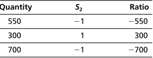
This indicates that the limit may be reducedby 300 pounds (down to zero pounds) without changing the solution.

The question asks if the resources can be increased to 400 pounds without affecting the basis. The smallest negative ratio (550) tells us that the limit can be raised to 850 pounds without changing the solution mix. However, the values of X1, X2, and S2 would change. X1 would now be 400, X2 would be 600, and S2 would be 450. This is best seen graphically in Figure 9.3.

550 1 550

300 1 300

(13)

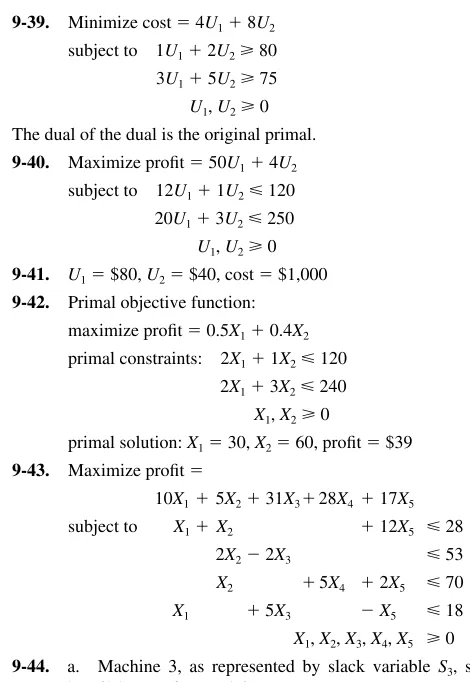
9-39. Minimize cost 4U18U2 subject to 1U12U280 3U15U275

U1, U20 The dual of the dual is the original primal.

9-40. Maximize profit 50U14U2 subject to 12U11U2120 20U13U2250

U1, U20 9-41. U1$80, U2$40, cost $1,000 9-42. Primal objective function:

maximize profit 0.5X10.4X2 primal constraints: 2X11X2120

2X13X2240

X1, X20

primal solution: X130, X260, profit $39 9-43. Maximize profit

10X15X231X328X417X5 subject to X1X2 12X5 28

2X22X3 53

X2 5X4 2X5 70

X1 5X3 X5 18

X1, X2, X3, X4, X5 0 9-44. a. Machine 3, as represented by slack variable S3, still

has 62 hours of unused time.

b. There is no unused time when the optimal solution is reached. All three slack variables have been removed from the basis and have zero values.

c. The shadow price of the third machine is the value of the dual variable in column 6. Hence an extra hour of time on machine 3 is worth $0.265.

d. For eachextra hour of time made available at no cost on machine 2, profit will increase by $0.786. Thus 10 hours of time will be worth $7.86.

9-45. The dual is

maximize Z120U1115U2116U3 subject to 8U1 4U29U323

4U1 6U24U318

U1, U2, U30

U1$2.07 is the price of each test 1

U2$1.63 is the price of each test 2

U3$0 is the price of each test 3 Using the dual objective function:

Z 120U1115U2116U3 120(2.07) 115(1.63) 116(0)

$248.4 $187.45 $0

$435.85

Thus $435.85 is the maximum the laboratory should be willing to pay an outside resource to conduct the 120 test 1’s, 115 test 2’s, and 116 test 3’s per day.

8U14U29U3is the value of 8, 4, and 9 of tests 1, 2, and 3, respectively, performed per hour by a biochemist. This means that the prices U₁, U₂, and U₃need to be such that their total value does not exceed the cost per hour to the lab for using one of its own biochemists.

Similarly, 4U1 6U2 4U3 is the value of 4, 6, and 4 of tests 1, 2, and 3, respectively, performed per hour by a biophysi-cist. Again, the prices U1, U2, and U3need to be such that the total value does not exceed the cost per hour for the lab to use one of its own biophysicists.

9-46. a. There are 8 variables (2 decision variables, 3 surplus variables, and 3 artificial variables) and 3 constraints. b. The dual would have 2 constraints and 5 variables (3 decision variables and 2 slack variables).

c. The dual problem would be smaller and easier to solve.

9-47. a. X127.38 tables, X2 37.18 chairs daily, profit $3775.78.

b. Not all resources are used. Shadow prices indicate that carpentry hours and painting hours are not fully used. Also, the 40-table maximum is not reached.

c. The shadow prices relate to the five constraints: $0 value to making more carpentry and painting time avail-able; $63.38 is the value of additional inspection/rework hours; $1.20 is the value of each additional foot of lumber made available.

d. More lumber shouldbe purchased if it costs less than the $1.20 shadow price. More carpenters are not needed at any price.

e. Flair has a slack (X₄) of 8.056 hours available daily in the painting department. It can spare this amount.

f. Carpentry hours range: 221 to infinity. Painting hours range: 92 to infinity. Inspection/rework hours range: 19Z\xto 41. g. Table profit range: $41.67 to $160 Chair profit range: $21.87 to $84.

9-48. Printout 1 on the right illustrates the model formulation (see the next page).

a. Printout 2 provides the optimal solution of $9,683. Only the first product (A158) is not produced.

b. Printout 2 also lists the shadow prices. The first, for example, deals with steel alloy. The value of one more pound is $2.71.

c. There is no value to adding more workers, since all 1,000 hours are not yet consumed.

d. Two tons of steel at a total cost of $8,000 implies a cost per pound of $2.00. It should be purchased since the shadow price is $2.71.

e. Printout 3 (also on the next page) illustrates that profit declines to $8,866 with the change to $8.88.

(14)

Problem Title: DATASET PROBLEM 9-48

***** Input Data *****

Max. Z 18.79X1 6.31X2 8.19X3 45.88X4 63.00X5 4.10X6 81.15X7 50.06X8 12.79X9 15.88X10 17.91X11 49.99X12 24.00X13 88.88X14 77.01X15

Subject to

C1 4X2 6X3 10X4 12X5 10X7 5X8 1X9 1X10 2X12 10X14 10X15 980

C2 .4X1 .5X2 .4X4 1.2X5 1.4X6 1.4X7 1.0X8 .4X9 .3X10 .2X11 1.8X12 2.7X13 1.1X14 400 C3 .7X1 1.8X2 1.5X3 2.0X4 1.2X5

1.5X6 7.0X7 5.0X8 1.5X12 5.0X13 5.8X14 6.2X15 600 C4 5.8X1 10.3X2 1.1X3 8.1X5 7.1X6

6.2X7 7.3X8 10X9 11X10 12.5X11 13.1X12 15X15 2500

C5 10.9X1 2X2 2.3X3 4.9X5 10X6 11.1X7 12.4X8 5.2X9 6.1X10 7.7X11 5X12 2.1X13 1X15 1800 C6 3.1X1 1X2 1.2X3 4.8X4 5.5X5

.8X6 9.1X7 4.8X8 1.9X9 1.4X10 1X115.1X12 3.1X13 7.7X14

6.6X15 1000

C7 1X1 0

C8 1X2 20

C9 1X3 10

C10 1X4 10

C11 1X5 0

C12 1X6 20

C13 1X7 10

C14 1X8 20

C15 1X9 50

C16 1X10 20

C17 1X11 20

C18 1X12 10

C19 1X13 20

C20 1X14 10

C21 1X15 10

Printout 1 for Problem 9-48

Printout 2 for Problem 9-48

***** Program Output *****

Final Optimal Solution at Simplex Tableau : 18

Z $9,683.228

Variable Value Reduced Cost

X 1 0.000 0.000

X 2 20.000 0.000

X 3 10.000 0.000

X 4 10.000 0.000

X 5 11.507 0.000

X 6 20.000 0.000

X 7 10.000 0.000

X 8 20.000 0.000

X 9 50.000 0.000

X10 20.000 0.000

X11 20.000 0.000

X12 54.946 0.000

X13 20.000 0.000

X14 12.202 0.000

X15 10.000 0.000

Constraint Slack/Surplus Shadow Price

C 1 0.000 2.712

C 2 113.866 0.000

C 3 0.000 10.649

C 4 0.000 2.183

C 5 258.885 0.000

C 6 8.530 0.000

C 7 0.000 1.324

C 8 0.000 46.187

C 9 0.000 26.455

C10 0.000 2.535

C11 11.507 0.000

C12 0.000 27.370

C13 0.000 34.041

C14 0.000 32.676

C15 0.000 11.749

C16 0.000 10.842

C17 0.000 9.374

C18 44.946 0.000

C19 0.000 29.243

C20 2.202 0.000

C21 0.000 48.870

(d) Cost is $2.00/lb for more steel; we should do it.

SOLUTIONS TO

INTERNET

HOMEWORK

PROBLEMS

9-49. Maximize 20X110X20S10S2 Subject to: 5X14X2S1250

2X15X2S2150

X1, X20

CjlSolution 20 10 0 0

0 S1 5 4 1 0 250

0 S2 2 5 0 1 150

Zj 0 0 0 0 0

(15)

The pivot column is the X1column.

d. Variable X1will enter the solution mix. Profit will in-crease $10 for each unit of this that is brought into the so-lution.

e. ratio for row 124/212; ratio for row 236/218. The pivot row is row 1 (it has the smallest ratio).

f. The variable in the pivot row will leave the solution mix. This is S1.

g. The ratio for the pivot row is 12, so 12 units of X1will be in the next solution.

h. The total profit will increase by ($10 per unit) (12 units)$120.

9-52. a. Maximize profit20X130X215X30S10S2

MA2MA3

Subject to: 3X15X22X3S1120 2X1X22X3S2A2250

X1X2X3A3180

X1, X2, X30

b. S1120; A2250; A3180; all others0. Profit 430M.

9-53. a. S112; X216; X14; all others0.

b. The dual prices are 0 for constraint 1 (department A), 3 for constraint 2 (department B), and 4.5 for constraint 3 (department C).

c. The company would be willing to pay up to the dual price for additional hours. This is $0 for department A, $3 for department B, and $4.50 for department C.

d. The profit on product #3 would have to increase by $1 (the negative of the CjZj value).

Printout 3 for Problem 9-48

Problem Title: DATASET PROBLEM 9-48

***** Input Data *****

Max. Z 18.79X1 6.31X2 8.19X3 45.88X4 63.00X5 4.10X6 81.15X7 50.06X8 12.79X9 15.88X10 17.91X11 49.99X12 24.00X13 8.88X14 77.01X15

***** Program Output *****

Final Optimal Solution At Simplex Tableau

Z $8865.500

Variable Value

X 1 0.000

X 2 20.000

X 3 10.000

X 4 16.993

X 5 7.056

X 6 20.000

X 7 10.000

X 8 20.000

X 9 50.000

X10 20.000

X11 20.000

X12 57.698

X13 20.000

X14 10.000

X15 10.000

CjlSolution 10 8 0 0

0 S1 2 1 1 0 24

0 S2 2 4 0 1 36

Zj 0 0 0 0 0

CjZj 10 8 0 0

9-50. The shadow prices are 3/10 for constraint 1; 0 for con-straint 2; and 3 for concon-straint 3. A zero shadow price means that additional units of that resource will not affect profit. This occurs because there is slack available. In this problem, constraint 2 has 425 units of slack (S2425), so additional units of this resource would simply increase the slack.

9-51. a. Maximize 10X18X2 Subject to: 2X₁1X₂24

2X14X236

X1, X20

b. S124; S226; X10; X20. Profit0. c.

Printout 4 for Problem 9-48

Final Optimal Solution at Simplex Tableau : 21

Z $9,380.234

Variable Value

X 1 0.000

X 2 0.000

X 3 0.000

X 4 0.000

X 5 28.723

X 6 20.000

X 7 10.000

X 8 37.517

X 9 50.000

X10 20.000

X11 33.941

X12 37.485

X13 20.000

X14 10.000