Creep Damage Calculation for Thermo Mechanical Fatigue

Creep Damage Calculation for Thermo Mechanical Fatigue

Šeruga, D. – Fajdiga, M. – Nagode, M. Domen Šeruga* _{– Matija Fajdiga – Marko Nagode}

University of Ljubljana, Faculty of Mechanical Engineering, Slovenia

For the needs of the creep damage prediction of thermo mechanically loaded components, software has been developed. It enables master curve determination using the time-temperature parameters and creep damage calculation using Robinson’s damage accumulation rule and simple time integration. The developed software makes it possible to calculate fatigue and creep damage, respectively. In the article the most used time-temperature parameters are introduced, a fast and user-friendly master curve determination is presented and an example of creep damage on a real set of data with a simple temperature-stress history is shown.

©2011 Journal of Mechanical Engineering. All rights reserved.

Keywords: creep, damage model, parametric methods, damage accumulation, Larson-Miller, Manson-Brown, Manson-Haferd, Orr-Sherby-Dorn, master curves

0 INTRODUCTION

Automotive components, gas and steam turbines, power plants and other products that operate at high temperature are subjected to creep. The lifetime of these components depends on thermal and mechanical loading. Typical examples are start-up, full load, partial load and shut-down [1]. The creep damage can no longer be neglected when the loading temperature exceeds the creep temperature typically determined as 40% of the melting temperature of the material [2] to [4]. Thus one of the critical factors in determining the lifetime of components is also their creep resistance. Due to the thermal loads materials slowly but constantly creep even at low mechanical loading, so rupture is possible. Rupture can be defined by some limit value of strain or by actual rupture depending on the type of component. It can be shown that the creep damage is determined by knowing the time to rupture depending on stress level and temperature.

1 MASTER CURVES

The criterion for creep damage calculation is given by master curves which represent time to rupture depending on stress level and temperature (Fig. 1). Each point on a master curve represents a complete creep-rupture test at constant temperature and stress level. As expected, higher test temperatures shift master curves towards lower stress levels and shorter times to rupture.

Master curve determination at lower stress levels and lower test temperatures usually means tests of very long duration, thus as a rule master curves in these areas are determined by using parametric extrapolation methods.

Fig. 1. Master curves

2 CREEP DAMAGE ACCUMULATION RULE

loading. Robinson proposed a linear creep damage accumulation rule [5]:

D t T

t T

ij ij ij ij ij ij j

m

i ni ij

c

r =

=

=

∑

∑

0

, (1)

where Δtij and trij are the actual times under some loading and temperature and the corresponding time to rupture at the same loading and temperature, respectively. Index i represents the number of the time step in load history and index

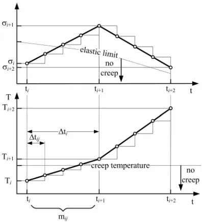
j represents additional subdivisions of time step i. Loading temperature T has to be higher or equal to creep temperature Tc and loading stress σ has to be higher than the temperature dependent elastic limit of the material k(T) otherwise, no creep occurs [2] to [4], (Fig. 2). If the loading temperature is beneath the limit temperature for which material data is available, then the material data for the limit temperatures is taken into account. The damage accumulation in a single time step is independent of the previously accumulated damage. When the sum of individual creep damages reaches the defined limit value (usually 1), creep rupture occurs. Robinson’s damage accumulation rule is the most widely accepted one [1], [3], [4], [6] to [8].

Fig. 2. Creep damage calculation

Creep damage is calculated as a simple integration over all the time increments according to Eq. (1) (Fig. 2). However, there are three

different creep relations used to calculate creep damage due to compressive stresses [4], [9] and [10]. The creep relation can allow either tensile creep only if:

0 < tr< ∞ if σ > k(T) and T > Tc, otherwise tr = ∞,

or tensile-compressive creep if:

0 < tr< ∞ if |σ|>|k(T)| and T > Tc,

otherwise tr = ∞,

or compressive healing if:

–∞ < tr < 0 if σ < –k(T) and T > Tc, 0 < tr < ∞ if σ > k(T) and T > Tc, otherwise tr = ∞.

The creep healing is possible only if

Dc(t) > 0. Moreover, the tensile-compressive creep is larger than or equal to the tensile creep that is larger than or equal to the compressive healing.

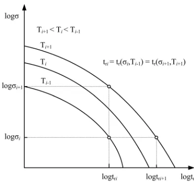
The appropriate creep relation depends on the material. Some materials tend to heal under compressive loading while for other materials creep damage continues to grow regardless of the direction of the loading. The influence of the creep relation on the creep damage accumulation is shown in Fig. 3. The temperature is supposed to be constant, while stress changes from tension to compression at t1. Before t1 the creep relation

does not affect Dc. However, after t1 the

tensile-compressive creep results in the highest Dc, while compressive healing in the lowest.

Fig. 3. Influence of the creep relation upon the creep damage accumulation

3 SPECIMENS, MATERIAL AND TESTING

3.1 Material

The material under investigation is 5Cr0.5Mo steel. It is suitable for components operating at high temperatures. Specimens with geometry of 6 mm in diameter and 30 mm in gauge length were taken longitudinally from the boiler tubes at the middle of the wall thickness.

3.2 Testing

Material is tested at temperatures of 500, 550, 600 and 650 ºC and at various stress levels with standard creep-rupture testing [ASTM E 139 – 00]. Every test is performed at a single temperature and a single load up to rupture. The specimen is loaded with a constant load. Time to rupture, area reduction at rupture and elongation at rupture are recorded.

3.3 Test Results

Test results are shown in Fig. 4. For extrapolation purposes one set of data is chosen. Since the main goal is to determine master curves from the shortest creep-rupture tests, results at the highest stresses and the highest temperatures

are selected. Results gained by extrapolation are compared with 4 comparison sets of experimental data. Each comparison set represents the results of creep-rupture testing at a distinct test temperature.

4 TIME-TEMPERATURE PARAMETERS

Time-temperature parameters represent a parametric method for determining time to rupture. The basic idea of every parametric method is to predict long-term creep behaviour by compensating time with temperature, i.e. to obtain long-term creep estimates from short-term tests at higher temperature at the same stress [12]. Time-temperature compensation parameters are introduced to establish a model for the estimation of long-term creep properties. Mostly used compensation parameters are introduced below. The assumption made at every extrapolation is that no change of metallurgical microstructure in the extrapolation space occurs. By applying proposed constitutive equations at every described parameter, a master curve is obtained (Fig. 1). Usually, a second degree polynomial sufficiently describes the master curve [13]. Coefficients used for every parameter are obtained by the least-squares method and are presented in the tables for

the data used. Master curves for the Larson-Miller parameter for four test temperatures are shown in Fig. 5. They are obtained exclusively from the data used for extrapolation (Fig. 4). However, it is possible to predict time to rupture for every stress and temperature.

4.1 Larson-Miller Parameter

The LM parameter [14] assumes that the logarithm of the time to rupture is inversely proportional to temperature.

LM = T(logtr + C), (2)

logt C log log

T a a a

r = − +1

(

)

Table 1. LM coefficients for used test results

C a0 a1 a2

19 18123 6715 -3264

4.2 Manson-Brown Parameter

The MB parameter [15] assumes that the logarithm of the time to rupture is a power function of temperature.

MB t t

T T q

= −

−

(

)

log r log a

a

, (4)

log log

log log

t t

T T q a a a

r a

a

= +

+

(

)

(

)

Table 2. MB coefficients for used test results

logta Ta q a0 a1 a2

-36.4 666.5 -0.143 79.9 18.2 -8.4

4.3 Manson-Haferd Parameter

The MH parameter [16] assumes that the logarithm of the time to rupture is proportional to temperature.

MH t t

T T

= −

−

log r log a a

, (6)

log log

log log

t t

T T a a a

r a

a

= +

+

(

)

(

)

Table 3. MH coefficients for used test results

logta Ta a0 a1 a2

-29.9 2242 -0.023 -0.006 0.003

4.4 Orr-Sherby-Dorn Parameter

The OSD parameter [17] assumes that the logarithm of the time to rupture is equal to the reciprocal value of temperature and risen for a constant.

OSD t A

T

=log r − , (8)

logt A log log

T a a a

r = + 0+ 1 σ+ 2 2σ. (9)

Table 4. OSD coefficients for used test results

A a0 a1 a2

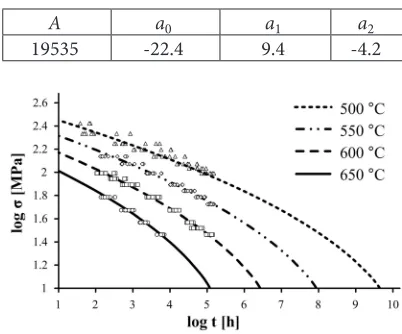
19535 -22.4 9.4 -4.2

Fig. 5. Master curve determination with the LM parameter; coefficients are gained exclusively

from the data used for extrapolation

4.5 Comparison of Time-Temperature Parameters

Time-temperature parameters are compared with the goodness of master curves’ fit for four comparison sets. Each comparison set has actual time to rupture values xai (Fig. 4). Predicted time to rupture values xpi are calculated from the data used for extrapolation (Fig. 4). E[xa] is the mean of actual time to rupture data for each comparison set. The residual sum of squares:

TSS=

∑

(

[ ]

)

, (11)

for each comparison set. By comparing the values

RSS and TSS, a value for goodness of fit M can be introduced, denoted by:

M RSS

TSS

x x

x E x

i i

i

i i

= − = −

(

)

−

[ ]

(

)

∑

∑

1 1

2

2

a p

a a

. (12)

If the predicted results are compared to the data used for extrapolation the M value will coincide with the R2 _{value [18]. However, the}

obtained R2 _{value could be negative for two}

different sets of data and its validity is therefore questionable (i.e. comparison set 1 and data used for extrapolation Fig. 4). The M value cannot be used to predict whether a model is good or not. But since it is the same measure for all compared parameters it gives an insight into which parameters are better than others. If the M value is near 1, the model seems to be acceptable for that comparison set. If it is 0 or even negative the model appears to be useless in that particular area. Goodness of fit calculated by the M value is given numerically in Table 5 and graphically in Fig. 6.

Table 5. Calculated M values for comparison sets with different time-temperature parameters

T [ºC] 650 600 550 500

Par. Comp. set 1

Comp. set 2

Comp. set 3

Comp. set 4

LM 0.936 0.922 0.718 0.810

MB 0.929 0.873 -1.871 -109.2

MH 0.931 0.887 0.951 0.201

OSD 0.918 0.796 0.872 0.847

Master curves gained by different time-temperature parameters look very similar at first sight but a detailed analysis (in this case with the M value) reveals a significant difference in assessment of the time to rupture. Assessment of the coefficients represents a significant challenge regardless of which time-temperature parameter is used.

The M value is comparable for LM-, MH- and OSD parameters (comparison sets 1 to 4). It can be noticed that the master curves are the most conservative when using the MH parameter, the least conservative when using the LM parameter;

the OSD parameter lies somewhere in between. The M value shows that the MB parameter is good only if the stress area is being extrapolated (comparison sets 1 and 2). If the MB parameter is used also for extrapolating results in the temperature area, the actual and predicted results deviate significantly (comparison sets 3 and 4). For extrapolation purposes a set of data at two highest temperatures and three highest stress levels were chosen. By this choice the creep-rupture testing would be the shortest. It can be proven that two stress levels or one test temperature alone are not sufficient for a reliable prediction of the time to rupture at unknown temperatures and unknown stress levels. If more test temperatures and more stress levels were taken into account for assessment of the time-temperature parameters the matching between actual and predicted times to rupture would improve. Despite less conservative predictions with the LM parameter its usage is more satisfactory as it is still one of the most used time-temperature parameters for determining the master curves [19] and [20].

Fig. 6. Calculated M values for comparison sets with different time-temperature parameters

(negative values are plotted as 0)

5 DETERMINATION OF COEFFICIENTS

a general form of the master curve equation. A second order polynomial is sufficient for the description of the master curve, thus the time to rupture using the LM parameter (Eq. (3)) can be written in the general form:

logt b br = 0+ 1logσ +b2log2σ , (13)

where b C a

T

0 = − + 0 , b1= a_T1 and b2 =a_T2 . Coefficients b0, b1 and b2 can be obtained easily

by drawing a trend line through the test data in any commercial software. The presented software calculates C, a0, a1 and a2 with the least-squares

method;

S

t C a

T a T a T ij j

j i j i j

m 2

0

1 2 2

1 = + − − − +             =

∑

∑

where n and m are the number of stress levels and the number of test temperatures, respectively. If Eq. (13) is taken into account Eq. (14) can be rewritten in the form:

S

b b b C

a T a T a T

j j i j i

j j i j i

2

0 1 2 2

0 1 2 2

= + + + − − − +     log log log log σ σ σ σ       = =

∑

∑

1 . (15)

Equalling partial derivatives of Eq. (15) with zero: ∂ ∂ = ∂ ∂ = ∂ ∂ = ∂ ∂ = S C S a S a S a 2 2 0 2 1 2 2

0; 0; 0; 0; (16)

the LM coefficients C, a0, a1 and a2 are obtained.

The same procedure may be used for every presented time-temperature parameter. Master curves with a temperature step ΔT = 10 ºC over the whole test area (500 to 650 ºC) are depicted in Fig. 7.

6 EXAMPLE OF CREEP DAMAGE CALCULATION

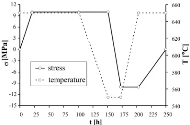
Creep damage calculation with Robinson’s damage accumulation rule and master curves determined by the LM parameter (Fig. 7) is performed on a simple temperature-stress history (Fig. 8).

Fig. 7. Master curves with a temperature step ΔT = 10 ºC over the whole test area (500 to 650 ºC)

Fig. 8. A simple temperature-stress history

The loading temperature is kept at 650 ºC at the beginning, decreases to 550 ºC after 150 h and increases back to 650 ºC after 200 h. Tensile loading stress rises to 10 MPa and remains constant for 150 h, then it turns into compressive direction with the same value. Creep damage calculation is performed online between successive time steps. Every time step is divided into smaller time sub steps. Their sizes depend on the stress or temperature jump in the actual time step. Creep damage is calculated as integration over all time steps and is depicted in Fig. 9. The thick line shows creep damage changing and the thin line shows the fatigue damage growing. The creep contribution to the damage of the thermo mechanically loaded component can be seen easily from the 20th _{to the 100}th _{hour where the fatigue}

damage remains constant due to constant loading conditions whereas creep damage constantly grows. From the 150th _{hour on, the influence of}

Fig. 9. Damage calculation for the simple temperature-stress history

7 SUMMARY AND CONCLUSIONS

The developed software makes separate and quick calculations of the creep damage possible if temperature dependent material parameters and temperature-stress history are known. For determination of the material parameters only a few standard creep-rupture tests at different test temperatures and different stress levels are required. Extrapolation of the material parameters is possible using any of the introduced time-temperature parameters. The input material data are always coefficients for every known master curve and in the software they are appropriately transformed regarding the selected time-temperature parameter. The next step in the development of the creep damage calculation will be a search for a generalized time-temperature parameter which would embrace the introduced time-temperature parameters into a single form. Once achieved, the creep damage calculation will be compared to the actual creep damage of the specimens at controlled loading conditions. The introduced programme code is also integrated into the commercial software LMS Virtual.Lab.

8 REFERENCES

[1] Granacher, J., Scholz, A., Möhlig, H. (2000). Behaviour of heat resistant power plant steels undergoing variable long term loading conditions. Mat.-wiss. u. Werkstofftech., vol. 31, p. 29-37.

[2] Lemaitre, J., Chaboche, J.L. (2000).

Mechanics of solid materials. Cambridge University Press, Cambridge.

[3] Wiswanathan, R. (1989). Damage

Mechanisms and Life Assessment of

High-Temperature Components. ASM

International.

[4] Kropiwnicki, J., Hack, M. (2006). Improved calculation of damage due creep by more accurate time to rupture data presentation.

Progressive Technologies, Engines and Mechanisms in Mechanical Engineering: Scientific Journal of the International Baltic Assocciation of Mechanical Engineers, Kaliningrad.

[5] Robinson, E.L. (1938). Effect of temperature variation on the creep strength of steels.

Trans. ASME, vol. 160, p. 253-259.

[6] Nagode, M., Hack, M. (2004). An online algorithm for temperature influenced fatigue-life estimation: stress-life approach.

Int. J. Fatigue, vol. 26, p. 163-171.

[7] Sabour, M.H., Bhat, R.B. (2008). Lifetime prediction in creep-fatigue environment.

Materials Science Poland, vol. 26, p. 563-584.

[8] Ainsworth, R.A., Budden, P.J. (1994). Design and assessment of components subjected to creep. Journal of strain analysis, vol. 29, p. 43-50.

[9] Wada, Y., Aoto, K., Ueno, F. (1996). Creep-fatigue evaluation method for type 304 and 316FRSS. International Atomic Energy Agency, p. 750-086.

[10] Jaske, C.E., Mindlin, H., Perrin, J.S. (1973). Combined low-cycle fatigue and stress relaxation of alloy 800 and type 304 stainless steel at elevated temperatures. Fatigue at Elevated Temperature, ASTM STP 520, p. 365-376.

[11] N. I. for Material Science, Creep Database. Retrieved on 15.9.2008 from https://tsuge. nims.go.jp/top/creep.html.

[12] Reti, T., Felde, I., Grum, J., Colas, R., Sarmiento, G.S., Moita de Deus, A. (2010). Extension of isothermal time-temperature parameters to non-isothermal conditions: Application to the simulation of rapid tempering. Strojniški vestnik - Journal of Mechanical Engineering, vol. 56, no. 2, p. 84-92.

creep-rupture data by means of least squares.

NASA MEMO 3-10-59E.

[14] Larson, F.R., Miller, E.J. (1952). Time-temperature relationship for rupture and creep stresses. Trans. ASME, vol. 74, p. 765-775.

[15] Manson, S.S., Brown, W.F. (1953). Time-temperature stress relations for correlation and extrapolation of stress rupture data.

Proc. ASTM, vol. 53, p. 683-719.

[16] Manson, S.S., Haferd, A.M. (1953). A linear time-temperature relation for extrapolation of creep and stress rupture data. NACA TN 2890.

[17] Orr, R.L., Sherby, O.D., Dorn, J.E. (1954). Correlations of rupture data for metals at elevated temperatures. Trans. ASM, vol. 46, p. 113-118.

[18] Motulsky, H., Christopoulos, A. (2004).

Fitting models to biological data using linear and nonlinear regression: a practical guide to curve fitting. Oxford University Press, Oxford.

[19] Kandare, E., Feih, S., Lattimer, B.Y., Mouritz, A.P. (2010). Larson–Miller failure modeling of aluminum in fire. Metallurgical and materials transactions A, vol. 41, p. 3091-3099.