University of New Orleans University of New Orleans
ScholarWorks@UNO
ScholarWorks@UNO
University of New Orleans Theses and
Dissertations Dissertations and Theses
5-22-2006
Target Detection Using a Wavelet-Based Fractal Scheme
Target Detection Using a Wavelet-Based Fractal Scheme
Gregory W. Stein
University of New Orleans
Follow this and additional works at: https://scholarworks.uno.edu/td
Recommended Citation Recommended Citation
Stein, Gregory W., "Target Detection Using a Wavelet-Based Fractal Scheme" (2006). University of New Orleans Theses and Dissertations. 437.
https://scholarworks.uno.edu/td/437
This Thesis is protected by copyright and/or related rights. It has been brought to you by ScholarWorks@UNO with permission from the rights-holder(s). You are free to use this Thesis in any way that is permitted by the copyright and related rights legislation that applies to your use. For other uses you need to obtain permission from the rights-holder(s) directly, unless additional rights are indicated by a Creative Commons license in the record and/or on the work itself.
TARGET DETECTION USING A WAVELET-BASED FRACTAL SCHEME
A Thesis
Submitted to the Graduate Faculty of the University of New Orleans
in partial fulfillment of the requirements for the degree of
Master of Science in
Engineering Electrical
by
Gregory W. Stein
Dedication
Acknowledgments
Contents
Abstract vii
List of Figures viii
1 Introduction 1
1.1 SAR and ATR . . . 1
1.2 Intensity-Based Features . . . 2
1.3 Textural-Based Features . . . 2
1.3.1 Previous Textural-Based Features . . . 2
1.3.2 The Proposed Wavelet/Fractal Feature . . . 3
1.4 Thesis Organization . . . 3
2 Background 5 2.1 Two Parameter CFAR . . . 5
2.2 The Extended Fractal (EF) Feature . . . 6
3 The Proposed Technique - Wavelet/Fractal Feature 8 3.1 Wavelet Definition . . . 8
3.2 Wavelet Transform, Roughness Feature, and Structure Function . . . 10
3.3 Average Weighted Roughness Feature . . . 13
3.4.1 Method 1 . . . 14 3.4.2 Method 2 . . . 15 3.5 Advantages of AR Feature . . . 15
4 Experimental Results 17
5 Conclusions 23
Bibliography 25
Appendix 31
Abstract
List of Figures
2.1 Annular window for calculation of CFAR feature . . . 6
3.1 Wavelet illustration . . . 9
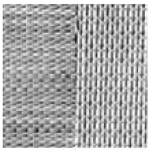
3.2 Texture sample . . . 11
3.3 Directional roughness feature illustration . . . 12
3.4 (a) Feature values around a target point, and (b) impulse response of matched filter . . . 13
4.1 Experimental Result 1 . . . 20
4.2 Experimental Result 2 . . . 21
Chapter 1
Introduction
1.1
SAR and ATR
1.2
Intensity-Based Features
Constant False Alarm Rate (CFAR) target detectors [2–8] have been developed in order to take advantage of the fact that the radar cross section of a target is higher than the surround-ing clutter. The two-parameter CFAR feature [2] is a computationally inexpensive clutter adaptive statistic, and for this reason is considered to be one of the benchmark algorithms for target detection. It assumes that the background clutter follows a Gaussian distribution. Other CFAR detectors have been developed [3–7] that consider more realistic clutter model distributions, such as Weibull. Rifkin [5] focuses on order statistic-based algorithms which calculate radar detection thresholds. These determine closed-form approximations for the signal-to-clutter ratio required to achieve a particular probability of detection in clutter en-vironments dominated by the Weibull distribution. Morgan et al [7] presents a technique for determining the ideal detection threshold when Gaussian noise and Weibull distributed clutter returns are present on a radar receiver and neither is dominant. Kaplan [9] mentions several techniques that search for objects only on the basis of contrast or intensity [10] may be problematic. In particular, several clutter objects included in SAR imagery (such as trees and buildings) may have intensities similar to that of the true targets.
1.3
Textural-Based Features
1.3.1
Previous Textural-Based Features
segmentation of clutter in high-resolution SAR imagery. The fractal dimension of natural clutter sources was used as an input to a Bayesian classifier. Scenes were segmented into three classes, namely shadows, trees, and grass. The relevance of the resulting segmentation maps to CFAR target detection techniques was also discussed. Kaplan [9] introduces a new feature, namely the Extended Fractal (EF) feature, to improve target detection performance. The EF feature is similar to the multiscale Hurst parameter used to measure multiscale texture roughness [14]. Comparisons illustrated that EF can provide a smaller number of false alarms than the contrast-only features, such as the two-parameter CFAR, for a specific detection rate.
1.3.2
The Proposed Wavelet/Fractal Feature
In this thesis, a wavelet-based fractal feature set for target detection is proposed. Both EF and the proposed feature sets attempt to exploit the textural characteristics of SAR imagery. However, Charalampidis has recently shown that a Wavelet/Fractal (WF) feature set [1], similar to the proposed one, provided lower classification error rates than a feature set similar to EF for a general texture classification problem. The promising performance of the WF features motivated the comparison presented in this thesis between the two techniques. It should be stressed that this thesis is not a direct implementation of Charalampidis’ WF feature [1]; furthermore, a heavily modified partition function is used for this SAR applica-tion, discussed in Chapter 3. Thus, this thesis concentrates on the development of a purely textural feature used to detect targets in SAR images.
1.4
Thesis Organization
Chapter 2
Background
In this chapter, the two-parameter CFAR and the EF feature are described. The first, CFAR, is presented since it is a commonly used feature for target detection, while the second, EF, can be considered a predecessor to the author’s feature set.
2.1
Two Parameter CFAR
The two-parameter CFAR feature used in SAR ATR systems [2] attempts to distinguish targets from clutter based on the idea that the image intensity corresponding to targets should be larger than that of the surrounding clutter. The feature is computed for each image pixel. In addition, CFAR assumes the background clutter follows a Gaussian distribution. Considering a pixel located at (m, n), CFAR is defined as the difference between the pixel value I(m, n) and the surrounding clutter normalized by the surrounding clutter standard deviation:
C(m, n) = I(m, n)−µˆ(m, n) ˆ
σ(m, n) (2.1) The values ˆµ(m, n), the clutter mean, and ˆσ(m, n), the clutter standard deviation, are esti-mated over a one pixel-wide square annular window containingNc elements around location
the length of the target to ensure that the window only includes pixels corresponding to clutter. The previous statement implies that some prior knowledge about the target’s size (in pixels) is required for this feature.
To illustrate the two-parameter CFAR feature, assume a target is within the annular
Test Target pixel
Annular window consisting of Nc pixels
Figure 2.1: Annular window for calculation of CFAR feature
dow. Based on the assumption that targets have higher intensity than surrounding clutter,
I(m, n)−µˆ(m, n), normalized by ˆσ, outputs a pixel with relatively high intensity. Thus, in the resultant image, the target locations have high intensity, and all surrounding pixels have much lower intensity. The CFAR algorithm presented in this section does not always perform as expected; in fact, it is accepted that CFAR produces a high false alarm rate, but it still considered a benchmark idea. However, the processing time for the CFAR algorithm is minimal.
2.2
The Extended Fractal (EF) Feature
The EF feature, unlike the CFAR feature, attempts to exploit the textural characteristics of the SAR images. Given a discrete image I(m, n), the x- and y-directed EF features are defined as the log ratio of the local average power considering lags 2∆ and 4∆ in the x- and y-directions, respectively:
Fx(m, n) = 1 2log2
fx
∆(m, n)
fx
2∆(m, n)
Fy(m, n) = 1 2log2
f∆y(m, n)
where fx and fy are called structure functions defined as:
f∆x(m, n) =
w
X
i=−w w
X
j=−w
|I(m+ ∆ +i, n+j)−I(m−∆ +i, n+j)|2 f∆y(m, n) =
w
X
i=−w w
X
j=−w
|I(m+i, n+ ∆ +j)−I(m+i, n−∆ +j)|2 (2.3) As Equation 2.3 describes, the structure functions are computed considering a sliding window of size W ×W, whereW = 2w+ 1 The window size W depends on the smallest lag so that
∆ = W −1
4 . (2.4)
Note that ∆ must be an integer so that the window size must equal one plus a multiple of four. To achieve directional invariance, the EF feature is defined as the average of the two directed features.
F(m, n) = Fx(m, n) +Fy(m, n)
Chapter 3
The Proposed Technique
-Wavelet/Fractal Feature
In this chapter, a new feature extraction technique used for target detection is presented. In this feature, fractal measures are computed using directional wavelets defined in the following sections [1].
3.1
Wavelet Definition
A wavelet, which is part of a larger fractal family, is simply a mathematical function that segments data into different components at a given scale s. For the purposes of this thesis, the wavelet needs to be viewed as a transition detector in the SAR images.
A two dimensional Gaussian smoothing function at scale s is defined: Φ(x, y, s) = e−x2+y
2
2s2 (3.1)
subscript indicates the wavelet direction angle.
W0(x, y, s) =
∂Φ(x, y, s)
∂x =−
x se
−x2+y2
2s2
W90(x, y, s) =
∂Φ(x, y, s)
∂y =−
y se
−x2+y2
2s2 (3.2)
A simple illustration for the 0◦-direction at scale 1.5 and 90◦-direction at scale 3 is shown in Figure 3.1:
(a) 0oWavelet – Scale 1.5 (b) 90oWavelet – Scale 3
Figure 3.1: Wavelet illustration
One may notice that the wavelets in Figure 3.1 are not normalized, indicating that the wavelet at scale 3 has much higher energy than the wavelet at scale 1.5. However, this phenomena does not need to be accounted for since computations only occur using one scale at a time.
Given an image I(x, y), and because differentiation and convolution are linear operators:
W0(x, y, s)∗I(x, y) =
∂Φ(x, y, s)
∂x ∗I(x, y) = ∂
∂x[Φ(x, y, s)∗I(x, y)] W90(x, y, s)∗I(x, y) =
∂Φ(x, y, s)
∂y ∗I(x, y) = ∂
Therefore, W0(x, y, s)∗ I(x, y) and W90(x, y, s) ∗ I(x, y) are the gradient components of
Φ(x, y, s)∗I(x, y) in directions 0◦ and 90◦, or the filtered versions of I(x, y) using filters
W0(x, y, s) and W90(x, y, s), respectively. Computation of the filtered image in an arbitrary
direction θ requires filtering the image I(x, y) by the wavelet Wθ(x, y, s) = W0(xcosθ +
ysinθ,−sinθ+ycosθ, s). The convolution Wθ(x, y, s)∗I(x, y) is the θ-directed gradient
component of Φ(x, y, s)∗I(x, y) along x0 =xcosθ+ysinθ and can be computed as a linear combination of the 0◦ and 90◦ components:
Wθ∗I(x, y) = [W0(x, y, s)∗I(x, y)] cosθ+ [W90(x, y, s)∗I(x, y)] sinθ (3.4)
Therefore,Wθ(x, y, s) is said to be steerable, andWθ(x, y, s)∗I(x, y) is computed for different
angles of θ from the 0◦ and 90◦ components using Equation 3.4. The steerability of the wavelet saves significantly in computation time because only two convolutions need to be computed for any filtering direction. As shown by Charalampidis [1], the second partial derivatives as well as higher order derivatives of the smoothing function can be considered; however, for the purposes here, only first order derivatives are considered.
3.2
Wavelet Transform, Roughness Feature,
and Structure Function
Consider the following wavelet transform of imageI(x, y) at scale s and direction θ:
W TIθ(x, y, s) =Wθ(x, y, s)∗I(x, y) (3.5)
Next the directional roughness features Rθs(x, y) are determined for every pixel by the fol-lowing power-law relation of the partition function µs,θ,,N(x, y):
where<>N×N indicates the spatial arithmetic average in aN×N window andA is defined
as an annular window of radius , similar to the one shown in Figure 2.1. In essence, the partition function is finding the difference between the maximum and minimum value in an annular window for each pixel in W Tθ
I(x, y, s). The directional roughness feature for each
image pixel is computed as the slope of the line that best fits (log,logµs,θ,,N(x, y)). This
implies thatis a vector considered for everyθ. The partition functionµs,θ,,N(x, y) of
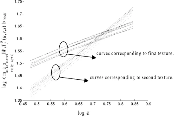
Equa-tion 3.6 is a modified version of the one used by Charalampidis in [1]. Figure 3.3 illustrates examples of such lines for the structure function originally proposed by Charalampidis [1] for two different textures, similar to those displayed in Figure 3.2, at different texture locations,
for s= 2, N = 9, θ = 0◦, and 832= [1 2 3]. Notice that lines extracted from different locationsIEEE TRANSACTIONS ON IMAGE PROCESSING, VOL. 11, NO. 8, AUGUST 2002
Fig. 8. Segmentation examples. The images namedor are the original images, while the images named seg are the corresponding segmented images.
pixel in this window has a different assigned classification. Es-sentially, ambiguous regions are the ones close to the cluster boundaries. The labels “A” and “U” indicate the pixel status, i.e., they suggest if the pixel should be reexamined (label “A”) or not (label “U”). This region marked “A” will be reexamined but the features will be smoothed with a smaller moving-average window.
Fig. 7(e) shows the segmentation result at a later stage. Here, some part of the “A” region has already been associated to the existing clusters. One can notice that the details at the bound-aries are better preserved. On the other hand, since the
moving-into consideration. For instance, the pixel at the center of the square window shown in Fig. 7(e) will be associated either to cluster 1 or to cluster 2, since cluster 3 is spatially far away (no pixel marked cluster 3 exists in this window). Fig. 7(f) shows the final segmentation, which is close to the ideal, in terms of boundary details.
The above algorithm is applied more than once for different selections of the initial centers to increase the probability of ap-proaching the global minimum. The criterion for determining which clustering is better is the minimization of the square error, which is equivalent to minimizing the quantity WCSS as it is
Figure 3.2: Texture sample
of the same texture are almost parallel to each other, which verifies the robustness of the directional roughness features, Rθ
s(x, y). The distance between lines corresponding to the
same texture can be accounted for due to contrast differences at various texture locations. Furthermore, the directional roughness feature is less sensitive to intensity and contrast dif-ferences within the same texture, which is advantageous when attempting to distinguish targets from clutter in SAR images.
Next, some intuition is provided to help understand the reasoning behind this particular partition function. First, it should be emphasized that the transform of Equation 3.5 is the θ-direction gradient component of the image I(x, y). This implies that high intensi-ties in W Tθ
I(x, y, s) correspond to sharp transitions in I(x, y). Thus, in general, transform
828 IEEE TRANSACTIONS ON IMAGE PROCESSING, VOL. 11, NO. 8, AUGUST 2002
Fig. 4. Examples of lines that best fit(log "; loghmax jW T (u; v; s)ji ) (s = 2; N = 9; = 0 ; " = 1; 2; 3) for two textures, at different texture locations.
Therefore, and are the gradient components of in directions 0 and 90 , respectively, or the filtered versions of using filters and , respectively. Computation of the filtered signal in an arbitrary direction requires fil-tering of by the wavelet
. The convolution is the -direction gradient component of
along , and can be computed as a linear combination of the 0 and 90 components
(8)
In other words, is steerable [17], therefore, is computed for different angles , from the 0 and 90 components using (8), which saves significantly in computation time.
Similarly, we can consider the second partial derivatives of the smoothing function
(9)
lution between and
can be computed using the components in (9)
(10)
We define the following two wavelet transforms of a function at scale and direction :
(first derivative wavelet)
(second derivative wavelet). (11)
We introduce the directional roughness features similarly to (4)
(12)
where indicates spatial arithmetic average in an window, and , (first and second derivative, respectively). The directional roughness features are computed as the slope of the line that best fits
Fig. 4 illustrates examples of such lines for two different tex-tures, at different texture locations, for , , ,
Figure 3.3: Directional roughness feature illustration
W Tθ
I(x, y, s) tends to highlight the target outlines, since moving from a target pixel to a
background/clutter pixel presents a sharp transition. At the same time, transform pixels inside and outside the target possess a low intensity. The partition function is essentially the average difference, in aN×N window, between the maximum and minimum intensities of the transform in an annular windowA of radius .
Let us consider the case where a pixel is located inside the target. If the value of is similar to the target’s radius, then A includes pixels from the outline, as well as from inside the
target, resulting in a large max-min difference. As increases A includes pixels only from
outside the target, resulting in a small max-min difference. Then, it is expected that, for pixels located inside the target, the max-min difference is decreasing as increases. This results in a negative exponent based on the definition of Equation 3.6. On the other hand, for pixels outside but relatively near the target’s outline, the difference is small for small
, since target outline pixels are not included in A, and increases as increases, since A
considered for illustration purposes. Therefore, Figure 3.4(a) depicts a high negative value at the target surrounded by moderate positive values around the target.
(a) (b)
Figure 3.4: (a) Feature values around a target point, and (b) impulse response of matched filter
3.3
Average Weighted Roughness Feature
Due to the visual effect of roughness being highly dependent on the relative textural energy between different directions, the roughness features, Rθ
s(x, y), described in the previous
sec-tion, must be weighted. For example, if a texture is rougher in direction θ1 than direction
θ2, but has less energy, direction θ1 may appear to be less rough than direction θ2. As a
result, Equation 3.7 describes apercentage of energy [1] feature computed in directionθ and scale s. The percentage of energy, P ersθ, is insensitive to both absolute image illumination since the DC component has been removed by the exponential wavelet and contrast changes since a change in contrast will multiplyEsθ and EsT otal by a common term.
P erθs = E
θ s
ET otal s
(3.7) where
Esθ =DW Tθ
I(x, y, s)
E
EsT otal =X θ D W T θ
I(x, y, s)
E
N xN (3.9)
Thus, aweighted roughness feature can be defined as the roughness featureRθ
s(x, y) weighted
with the percentage of energy with the same scale and direction:
W Rθs =RθsP erθs (3.10) Finally, to obtain a rotationally invariant feature, an average weighted roughness feature is introduced:
ARs=
1
Q X
θ
W Rθs (3.11) where Q is the total number of directions considered.
3.4
Filter Optimization
3.4.1
Method 1
As stated in Section 3.2, the general shape of a target’s roughness feature is known to roughly follow the Gabor function; thus, a filter of the form,
h(x, y) = cos(ω0
q
x2+y2)e−x2+y
2
2σ2 (3.12)
illustrated previously in Figure 3.4 can be considered a matched filter to the target. Figure 3.4(a) is the resultant image when the author’s feature is applied to a T72 battle tank from the MSTAR database. Notice that this roughly follows the shape of Figure 3.4(b), which was created using Equation 3.12 with ω0 = 0.06π and σ at the desired scale. These images
can be used to enhance the feature space by emphasizing target parts by filtering ARs with
3.4.2
Method 2
Assuming that training data is available and an array of possible targets is known, an improved optimization technique can be utilized. Given target images, T(x, y), an average can computed at scale s for all possible targets in a particular clutter image described by:
h(x, y) = 1
P X
T
ARTs(x, y) (3.13) where P is the total number of targets considered. It should be noted that for the experi-mental results presented in this thesis, Equation 3.13 is used since the targets in a particular clutter image are known. However, Equation 3.12 is also applied and performs quite well as a matched filter.
3.5
Advantages of AR Feature
The advantages of the author’s AR feature over the EF feature are discussed herein. First, AR uses a partition functionµs,θ,,N(x, y) that employs the smoothing function of Equation
3.1. Therefore, µs,θ,,N(x, y) is less sensitive to noise than other techniques, such as CFAR,
that do not use any type of smoothing. Second, µs,θ,,N(x, y) is computed using steerable
filters, and thus, roughness features can be computed in several directions with a relatively small computational overhead. As a result, it is expected that the average roughness features are less sensitive to target rotations compared to the EF features, which are computed as the average of only two directed features. Third, the proposed features are designed to detect target-like objects that are characterized by sharp transitions. This is a result of using the gradient-based filter. Finally, it appears that the proposed features provide better spatial resolution capabilities. More specifically, the feature mapARs(x, y) is an image of the same
Chapter 4
Experimental Results
In this chapter, comparisons between the proposed AR feature and the EF feature are presented. The comparisons are performed primarily in terms of the ability to visualize the difference between the feature values corresponding to targets and clutter in the feature-map images. Furthermore, a quantitative, statistical approach has not been used to determine the percentage of targets detected.
A number of example SAR images have been tested. These images consist of a mixture of clutter and targets, obtained from the MSTAR database. The targets, including their shadows, are artificially inserted into the clutter images using Adobe Photoshop. Thus, the target locations are known. It should be noted that Kaplan has used a similar technique in [9]. Three of the examples for which the two features were compared are shown in Figures 4.1, 4.2, and 4.3. From these figures, it can be observed that the images appear to be realis-tic. For Figures 4.1, 4.2, and 4.3, (a) is the original image, and (b) is the original image with target markers. Figures (c) and (d) portray the feature maps for the AR and EF features respectively.
re-duce the false alarm rate. However, it is not expected that the percentage of false alarms can be reduced down to zero. In order to achieve a near-zero false alarm rate, a subse-quent target/clutter recognition stage is necessary. If performed, the recognition step would attempt to classify targets and clutter into different categories and at the same time to eliminate any remaining false alarms. Nevertheless, since the recognition stage is time con-suming, it is important to be able to reduce the target search space. This can be achieved by a target/clutter detection process such as the one proposed in this work.
For the three subsequent comparisons, the following AR feature parameters were applied on an image downsampled at a 2:1 ratio:
• N = 19
• = [7 11 15]
• θ = [0◦ 45◦ 90◦ 135◦]
• s= 1.5
Similarly, the following EF feature parameters were applied on the same downsampled im-ages:
• ∆ = 7
• W = 4∆ + 1 = 29
correspond-high AR feature values at the corresponding locations in the feature map should be expected. Figure 4.1(d) depicts the EF feature map. It is apparent that the EF feature may result in more potential false alarms compared to the AR feature. Although the target locations correspond to relatively large EF feature values in the EF feature map, there are many clutter-associated locations with significantly high EF feature values. In particular, it can be seen in Figure 4.1(d) that the rightmost target may not be easily detected using a thresh-olding technique, since there are many other locations in the feature map with significantly higher EF values that do not actually correspond to a target. It should be mentioned that the EF features maps were contrast-enhanced in order to emphasize large feature values for illustration purposes. The example presented in Figure 4.2 may result in conclusions similar to Figure 4.1. In this case, AR clearly shows the 4 target locations, while EF shows a sig-nificant number of potential false alarms.
(a) Original image, (b) original image in which targets are marked, (c) feature map extracted using the proposed technique, (d) EF feature map
(a) (b)
(c) (d)
(a) Original image, (b) original image in which targets are marked, (c) feature map extracted using the proposed technique, (d) EF feature map
(a) (b)
(c) (d)
(a) (b)
(c) (d)
(a) Original image, (b) original image in which targets are marked, (c) feature map extracted using the proposed technique, (d) EF feature map
Chapter 5
Conclusions
A new feature extraction technique has been presented for target detection. This work was concentrated in the textural aspects of detection. It is of course understood that additional, non-textural features can be used in order to achieve an improved target detection perfor-mance. The author presents a new improved feature extraction scheme based on fractal dimension, and discusses why this is a promising feature. The presented results mostly illus-trate the feature’s potentials for detecting targets and distinguishing them from clutter. It can be observed that the proposed feature gives a relatively clearer indication of the targets’ locations compared to the EF feature.
Bibliography
[1] D. Charalampidis and T. Kasparis. Wavelet-based rotational invariant roughness fea-tures for texture classification and segmentation. IEEE Transactions on Image Process-ing, 11(8):825–837, August 2002.
[2] L. M. Novak, S. D. Halversen, G. J. Owirka, and M. Hiett. Effects of polarization and resolution on SAR ATR. IEEE Transactions on Aerospace and Electronic Systems, 33:102–116, January 1997.
[3] G. B. Goldstein. False alarm regulation in log-normal and Weibull clutter. IEEE
Transactions on Aerospace and Electronic Systems, 9(1):84–92, 1973.
[4] S. Kuttikkad and R. Chellappa. Non-gaussian CFAR techniques for target detection in high resolution SAR images. IEEE ICIP 94, pages 910–914, November 1994.
[5] R. Rifkin. Analysis of CFAR performance in Weibull clutter. IEEE Transactions on
Aerospace and Electronic Systems, 30(2):315–329, April 1994.
[6] V. Anastassopoulos and G.A. Lampropoulos. Optimal CFAR detection in Weibull
clut-ter. IEEE Transactions on Aerospace and Electronic Systems, 31(1):52–64, January
1995.
[7] C.J. Morgan, L.R. Moyer, and R.S. Wilson. Optimal radar threshold determination in Weibull clutter and Gaussian noise. IEEE Transactions on Aerospace and Electronic
[8] L. M. Novak and S. R. Hesse. On the performance of ordered-statistics CFAR detectors.
Proceedings of the 25th Asilomar Conference on Signals, pages 835–840, 1991.
[9] L.M. Kaplan. Improved SAR target detection via extended fractal features. Proceedings
of SPIE, 2755:58–69, April 1996.
[10] J.S. Salowe. Very fast SAR detection. IEEE Transactions on Aerospace and Electronic
Systems, 37(2):66–75, April 2001.
[11] N. S. Subotic, B. J. Thelen, J. D. Gorman, and M. F. Reiley. Multiresolution detection of coherent radar targets. IEEE Transactions on Image Processing, 6:21–35, January 1997.
[12] Q. Pham, T. M. Brosnan, and M. J. T. Smith. Multistage algorithm for detection of targets in image data. Proceedings of SPIE, 3070:66–75, April 1997.
[13] C.V. Stewart, B. Moghaddam, K.J. Hintz, and L.M. Novak. Fractional brownian motion models for synthetic aperture radar imagery scene segmentation. Proceedings of IEEE, 81(10):1511–1522, October 1993.
[14] L.M. Kaplan. Extended fractal analysis for texture classification and segmentation.
Appendix
Matlab Code
Three different MATLAB .m files are attached:
• FeatObt.m - Algorithm which calculates the average weighted roughness feature de-scribed in Chapter 3.
• wavefeat.m - Algorithm which outputs the directional roughness feature described in Chapter 3
5/11/06 10:00 PM D:\GWS\Thesis\03_22_2006\SPIE Target Detection\FeatObt.m 1 of 1
% Implementation of the Wavelet/Fractal feature presented in
% Gregory W. Stein's thesis, titled "Target Detection Using a Wavelet % Based Fractal Scheme
clear all, close all, clc
% Read SAR image file='Clutter4.bmp';
fprintf('Image Read...\n'); n_rows = 1474;
n_cols = 1784;
% Parameters - Window size, epsilons, and thetas considered N=9;
e=[7 11 15];
theta = [0 45 90 135];
% Determine roughness feature at a specified scale s=1.5; % Define scale
for i=1:length(theta)
[FV(:,:,i) EN(:,:,i) mag] = wavfeat(file,s,N,e,theta(i),n_rows,n_cols); fprintf('Angle %d...\n',theta(i));
end
fprintf('Scale Done...\n\n');
% Determine percentage of energy for i=1:length(theta)
PER(:,:,i) = EN(:,:,i)./sum(EN,3); end
% Compute weighted roughness feature WR = FV.*PER;
% Compute average weighted roughness feature AF = sum(WR,3)/length(theta);
% Create omni-directional wavelet - Gabor - Filter optimization N=25;
x=[-N:N]; x=repmat(x,[2*N+1 1]); y=[-N:N]'; y=repmat(y,[1 2*N+1]); s=12;
Wo = cos(2*pi*0.03*sqrt(x.^2+y.^2)).*exp(-(x.^2+y.^2)/(2*s^2)); % Matched Filter
% Optimize with "matched" filter AFf=filter2(Wo,AF);
4/12/06 3:14 PM D:\GWS\Thesis\03_22_2006\SPIE Target Detection\wavfeat.m 1 of 2
function [FV,FVEng,mag]=wavfeat(filename,s,N,e,ang,n_rows,n_cols) % [FV FVEng] = wavefeat(filename,s,N,e,ang)
% filename: image filename % s: wavelet scale - scalar % N: size of wavelet window % e: feature epsilon(s) - vector % ang: feature direction - scalar
% n_rows: number of rows in image - scalar % n_cols: number of columns in image - scalar
% Read and display target
mag = double(imread(filename)); mag=mag(1:2:end,1:2:end);
% Create n-exponential wavelet x=[-N:N]; x=repmat(x,[2*N+1 1]); y=[-N:N]'; y=repmat(y,[1 2*N+1]);
% Define "root" wavelets
W0 = (-x/s).*exp(-(x.^2+y.^2)/(2*s^2)); % Wavelet 0 degree W90 = (-y/s).*exp(-(x.^2+y.^2)/(2*s^2)); % Wavelet 90 degree
% Filter image with wavelet, take absolute value if ang == 0
F = abs(filter2(W0,mag)); % 0 degree elseif ang == 90
F = abs(filter2(W90,mag)); % 90 degree else
F = abs(filter2(W0,mag)*cos(ang*(pi/180)) + filter2(W90,mag)*sin(ang*(pi/180))); % Any angle
end
M = 19; % Filter window size for moving average % Directional roughness feature
for i=1:length(e) Msize = 2*e(i)+1;
maxmask = ones(Msize,Msize); maxmask(2:end-1,2:end-1) = 0; rnk=sum(sum(maxmask));
FMax(:,:,i) = log(ordfilt2(F,round(rnk*1),maxmask)-ordfilt2(F,round(rnk*0+1), maxmask)+0.0010);
FMax(:,:,i) = filter2(ones(M)/(M^2),FMax(:,:,i)); end
% Determine slope [P Q] = size(mag);
le = reshape(log(e),[1 1 length(e)]); % x-axis st1 = repmat(le-mean(le,3),[P Q 1]);
4/12/06 3:14 PM D:\GWS\Thesis\03_22_2006\SPIE Target Detection\wavfeat.m 2 of 2
4/12/06 3:14 PM D:\GWS\Thesis\03_22_2006\SPIE Target Detection\EF_Final.m 1 of 1
% Implementation of the Extended Fractal Feature from
% "Improved SAR Target Detection via Extended Fractal Features % by Lance M. Kaplan
% Read and display target;
mag=double(imread('Clutter4.bmp'));
% Down-sample Image --- I = mag(1:2:end,1:2:end);
% Apply EF Feature --- D = 7; % Delta
W = 4*D+1; % Filter window size % FE in x-direction
Ifiltx1 = filter2(ones(W,W),(abs(filter2([1,zeros(1,2*D-2),-1]',I))).^2); % FE in y-direction
Ifilty1 = filter2(ones(W,W),(abs(filter2([1,zeros(1,2*D-2),-1],I))).^2);
D1 = 2*D; % 2xDelta % FE in x-direction
Ifiltx2 = filter2(ones(W,W),(abs(filter2([1,zeros(1,2*D1-2),-1]',I))).^2); % FE in y-direction
Ifilty2 = filter2(ones(W,W),(abs(filter2([1,zeros(1,2*D1-2),-1],I))).^2);
Fx = 0.5*log2(Ifiltx1./Ifiltx2); % Ratio in x-direction Fy = 0.5*log2(Ifilty1./Ifilty2); % Ratio in y-direction F = (Fx + Fy)/2; % Average
figure(1),imshow(mag/255)