Modified-Decoupled Net Present Value: The Intersection of
Valuation and Time scaling of Risk in Energy Sector
Ali Shimbar, Seyed Babak Ebrahimi*
Faculty of Industrial Engineering, K. N. Toosi University of Technology, Tehran, Iran.
Received: 3 July 2017 /Accepted: 11 November 2017 Abstract
Although the practical importance of investment analysis in long-term energy investments is well understood, choosing the proper method has always been a dilemma. In this regard, classic evaluation methods, with a history of almost a century, are mostly favored, but using them in the valuation of long-lasting energy projects has particular shortcomings, nevertheless. The drawbacks mainly stem from two structural problems: a) reflecting risk in rate of return instead of cash flow thus summing up risk and time value of money in a single parameter, b) generalizing the predefined rate of return to all project life time regardless of changing nature of risk. To overcome such drawbacks, a new easy-to-implement method termed Modified-Decoupled Net Present Value (M-DNPV) is proposed that intercepts coupling of risk and time value of money by deducting the risky portion of expected cash flows. To cover the dynamic nature of risk and as a buffer against uncertainty, it is suggested to attribute measured risks to investment lifespan using an "uncertainty coefficient”. Finally, the ability of the new method is shown through a complicated energy investment: an Iranian Petroleum Contract (IPC).
Keywords: Energy investment, Decoupled NPV, Investment decision analysis, Project valuation, Net present value, Iranian Petroleum Contract.
1. Introduction
As the world becomes more technology dominated, the need for energy is becoming more pressing. Therefore, it is a must to plan for increasing energy demand and to invest more in energy projects. However, with the world at current economic and political turmoil, investors have to be more careful in decisions regarding investing in a long-term energy project, especially in developing countries where energy demand is projected to grow exponentially. It is by no means clear that initial investment analysis plays a notable role in success or failure of an investment and can directly affect the decision-making process. Hence, to achieve more definitive results, the analysis must be done with regard to risks and uncertainties associated with future cash flows. In other words, project valuation method and risk measurement techniques are the twin pillars of the financial process of determining whether or not a project should be pursued. Therefore, they have to yield a reliable yet understandable result.
The most popular method to value a project is Net Present Value (NPV) based on Discounted Cash-Flow (DCF) criteria. Although the DCF techniques were not first applied to non-financial
investments, nowadays they are widely being used by decision-makers. Nevertheless, using these methods in real investments, especially in the big ones in energy sector, is not straightforward due to the uncertainty of contributory factors. For instance, such techniques require the project cash flows to be assumed certain, whereas this is rarely the case in real world situations (Miller and Park, 2002). In most cases expert judgment is used to assess investment risks based on which engineering economists adjust project rate of return to cover systematic and non-systematic risks. The obtained rate is referred as hurdle rate or risk-adjusted discount rate (RADR) in the literature. By applying hurdle rate or risk-adjusted rate to evaluation, it is already assumed that all technical and financial risks have the same nature, and more importantly, time value of money and risk are interchangeable matters.
Espinoza and Morris (2013) substantiate the inconsistency of such assumptions, and introduce a new method termed Decoupled Net Present Value (henceforth DNPV) based on risk pricing. DNPV is basically derived from Certainty Equivalent Method (CEM). While, DNPV by considering the disparity between time value of money and risk offers a better methodology to quantify the true value of a project, it assumes that risks are constant during project life time and neglects the uncertainty. According to a comprehensive research for the performance of 365 megaprojects by Ernst and Young (2015), about 64 percent of projects fail to meet approved budgets. The very research emphasizes the need for a new approach that accounts for lack of certainty in the capital budgeting. Addressing this issue, the present study attempts to modify Decoupled NPV by the use of “uncertainty coefficient” to cover the changing nature of risk; such modification can somehow close the gap between risk and uncertainty in economic evaluation of energy projects. Also, it can link evaluation with reliable risk assessment practices to yield a better estimation of project value.
The main objectives this paper seeks to reach are: firstly, a better measurement of risk and uncertainty thus defining special insurance products to cover risks and as a buffer against uncertainties; secondly, performing a reliable valuation of long-lived risky energy projects by considering risk in cash flow. Hence, the paper tries to suggest a comprehensive method consistent with long-term nature of energy investments.
In the new proposed method labelled Modified-Decoupled Net Present (hereafter M-DNPV) the key variables to assess risks and uncertainties are identified at first then proper synthetic insurance packages will be defined to safeguard investment from unfavorable future changes. M-DNPV method is consisted with PMBOK (2013) as it starts with risk identification; after assessing and pricing identified risks M-DNPV has to seek answer for two important questions: (i) what is the real source of risk and where should it be reflected? (ii) How to deal with uncertainties over project life time? These questions display the main ideas as well as novelty of the proposed method, answering which covers the drawbacks in the previous works done on the basis of reflecting risk in project cash flow such as Espinoza (2014), and also it pushes the applicatory of CEM a step forward. Therefore, this research attempts to contribute to empirical literature by introducing a new complementary to DNPV which can suggest a framework that can take the effort out of analyzing of long-term energy investments.
2. Review
At the heart of investment theory lies the NPV method, which traces its origin back to Fisher (1930). Later, NPV became widely used in economic evaluation of real projects especially by Dean (1951). However, the traditional forms of NPV (and its close relative, the internal rate of return) have some drawbacks in dealing with today’s long-term energy projects. As a good example, Shimbar and Ebrahimi (2017) show that how using such approach can hinder proper allocation of financial resources to renewable energy sector. As for another example, Chiaroni et al. (2016), through an empirical study involving 130 Italian industrial companies, show that using classic methods may show that some energy efficiency technologies, such as combined heat and power (CHP) plants, electric motors, variable speed drives (VSD), and uninterruptible power supply (UPS), are not suitable which are in fact economically viable. This is can be mainly due to the current ways of incorporating risk and uncertainty into valuation.
The common practice to account for project risks is to use a risk-adjusted discount rate (RADR). To have RADR calculated, at first, the required rate of return is calculated using common methods such as WACC or Sharpe (1964) CAPM, then a particular premium is added to proxy the risky portion of project (see Damodaran (2012)). However, such approach has widely been challenged in the literature, for instance (Bhattacharya, 1978; Fama, 1977; Halliwell, 2001; Myers and Turnbul, 1977; Schmalensee, 1981). The procedure is mainly criticized due to the narrow conditions that must be fulfilled in order to perform a valid valuation. For example, risk must be constant and interchangeable with time value of money, also systematic and non-systematic risks must be reconcilable. Moreover, uncertainty is an integral element of capital budgeting, but adjusted-discount-rate approach cuts-off uncertainty from its real source which is cash flow (Carmichael, 2016). Furthermore, augmenting discount rate to cover the riskiness of a project is somehow a qualitative approach which may vary from investor to investor (Baker and Fox, 2003). Ultimately, using classic NPV reduces the impact of future cash flows, as the denominator in formula grows exponentially over time which can be a problem in long-term energy projects. While most of the inconsistencies regarding classic NPV method in conjunction with risk-adjusted discount rates have been widely highlighted in the literature, the classic NPV continues to be widely utilized in long-term energy investments analysis (Block 2007; Fox, 2011).
Robichek and Myers (1966 ) and Fama (1977) were among the first supporters of the idea of reflecting risk in cash flows. They pointed out some conceptual problems in using RADR as it sums up time value of money and risk in one number. They argue that since time and risk, basically, do not have a same nature, they must be separated in NPV method. Their proposed approach termed Certainty Equivalent Method (CEM) was basically derived from two basic questions: firstly, "What is the smallest certain return for which investors would exchange expected return?", and secondly, "What is the greatest amount investors would pay now in order to receive a certain return at time t?" The answer to the first question is certainty equivalent of return which will make the investor indifferent to receiving the risky return. The amount asked in the second question is actually the certain return discounted by risk-free rate. The certainty equivalent framework calculates the present value of future uncertain cash flow as follows:
𝑃𝑉 = ∑ 𝑅𝑡∗ (1+𝑖)𝑡 𝑛
𝑡=1 = ∑
𝛼𝑡𝑅̃𝑡 (1+𝑖)𝑡 𝑛
𝑡=1 = ∑
𝑅̃𝑡
(1+𝑘)𝑡
𝑛
𝑡=1 (1)
in Equation(1), 𝑅̃𝑡 is the expected future cash flow, 𝑅𝑡∗ is the certainty equivalent of 𝑅̃𝑡, 𝑘 is risk-adjusted discount rate, 𝑖 is risk-free rate and αt is the ratio 𝑅𝑡∗⁄𝑅̃𝑡 which converts the uncertain cash-flow to a certain one. αt in Equation(1) is defined as follows:
𝛼𝑡 = (1+𝑖)𝑡
(1+𝑘)𝑡 (2)
as, in Equation(2), k > i therefore αt will be always a number between zero and 1, which means it is originally a reducing factor. In fact, by αt𝑅̃𝑡 the uncertain part of cash flow is isolated and the rest is discounted by risk-free rate of return. Thus, we can consider αt as an uncertainty or a risk proxy related to each period. But, since 0 < αt< 1 then:
𝑙𝑖𝑚
𝑡→∞𝛼𝑡 = 𝑡→∞𝑙𝑖𝑚 (1+𝑖)𝑡
(1+𝑘)𝑡= 0 (3)
which means αt is paradoxically going to reduce over time. However, this cannot be true since in most cases uncertainty grows over time. Despite its robustness and flexibility, CEM Method has no practical manner for quantifying αt and the practical limitations caused CEM application to be limited. Espinoza and Morris (2013) best represent the fundamental concepts of CEM and propose a practical approach to calculate αt through risk pricing. According to this method, called Decoupled NPV (DNPV), cost of risks for each period are calculated then such amounts are subtracted from net cash flows. By having risks considered in cash flows, a risk-free discount rate can be used to calculate decoupled net present value.
Using cost of risk as a reduction factor and thereby converting a risky cash flow to a risk-free one is a practical approach, but considering risk as a constant parameter has the same drawbacks of applying a fixed rate of return. In today’s uncertainty driven world, all the things vary over time and from situation to situation thus risk is a dynamic matter. As a result, an investor ought to be thinking of changing nature of risk and even the growth of uncertainty over time. Therefore, there are still some work required to reach a comprehensive valuation method, and DNPV method needs specific complementary to be more precise and reliable.
3. Modified-Decoupled Net Present Value (M-DNPV)
The proposed M-DNPV method derives from defining synthetic insurance packages. These especial insurance products can guarantee the profitability of investment and can be applied to project cash flows. Hence, M-DNPV of a project can be calculated by discounting risk-free expected cash flows and is mathematically calculated by the formula below:
𝑀𝑁𝑃𝑉(𝑅̃, 𝐸,̃ 𝑖, 𝑄̃) = ∑ 𝑅̃𝑡−𝑄̃𝑅𝑡
(1+𝑖)𝑡 −
𝐸̃ 𝑡+𝑄̃𝐸𝑡 (1+𝑖)𝑡 𝑛
where the parameters 𝑅̃ and 𝐸̃ are expected revenues and estimated expenditures, respectively. 𝑄̃ denotes the price of synthetic insurance products which are in fact risk premiums regarding incomes and costs (𝑄̃𝑅𝑡 and 𝑄̃𝐸𝑡). In Equation 4, 𝑖 in the denominator indicates appropriate discount rate and as the risky portion of the cash flow is deducted therefore the risk-free discount rate must be applied.
The risk-free rate is the rate at which company can be sure that it would not lose any money, and generally, the rates of fixed income securities are served as it. Owing to the fact that financial choices play a vital role in business decisions, especially in tenders, neglecting the way of financing project cannot be true because different companies have different access to financial resources, and leverage is an important competition advantage. Therefore, prior to M-DNPV analysis, the financial capability of the project must be evaluated using common methods like WACC or MIRR (without considering risk). After being assured of the financial ability of the project, the M-DNPV will be used to value the real worth of the project by considering its risk aspects and uncertainty coefficients.
To have reliable synthetic insurance products which can safeguard investment from any negative changes in the future, risk premiums (𝑄̃𝑅𝑡 and 𝑄̃𝐸𝑡) must be calculated with regard to uncertainty. This necessitates the need for introducing uncertainty coefficient in pricing synthetic insurance products.
3.1. Uncertainty coefficient
There is always uncertainty about future changes and the behavior of decisive factors over time. Generally speaking, uncertainty has two major parts: a tangible part and an abstract one. Using historical data, investors can somehow measure the tangible part by calculating the probability of previous changes which is known as “risk”. In fact, risk is a specific portion of uncertainty that can be quantified, but the rest of uncertainty, not precisely known, still remains (Booker and Rossb, 2011). In other words, risk applies to situations where the odds of possible outcomes are known or can be estimated (Mian, 2011). However, uncertainty refers to situations where our knowledge is limited and we are not able to designate stringent probabilities (Knight, 1921). This is particularly true of long-term energy projects
In the new M-DNPV method, the identified risks are calculated in a particular period (normally one year) then this number is attributed to later periods using “uncertainty coefficient”. It is crystal clear that, in the new method, rate of return is an output not input, also it can be seen that larger risk results in a lower rate of return, which is in contrast with classic NPV where higher risk means higher rate of return.
“Uncertainty coefficient” in M-DNPV methodology is computed by the use “Modified-Square Root of Time Rule” (M-SRTR) introduced by Wang, Yeh, and Cheng (2011). The raw Square Root of Time Rule (SRTR) is a common method to deal with time scaling of risk where risk is time aggregated. Based on this rule, risk estimates are scaled to time horizons using √𝑡. The SRTR is already being used in Black-Sholes option pricing model where the volatility is given by 𝜎√𝑡, also, it is advocated by regulators like Basel Committee on Banking Supervision, and European Banking Authority. Although the SRTR is popular in dealing with time scaling of risk, there are different factors that contribute to raw SRTR scaling distortions such as serial dependence, heavy-tailedness, jumps, and volatility clustering. Wang et al. (2011) empirical study shows that time dependence is more relevant, thus to mitigate its effect they suggest a Modified-SRTR based on variance ratio test.
𝑉𝑅
̅̅̅̅(𝑡) = 1 + 2 ∑ (1 −𝑘 𝑡) 𝑡−1
𝐾=1 𝜌̂𝑘 (5)
where 𝜌̂𝑘is the kth order autocorrelation coefficient of data series. When 𝑉𝑅̅̅̅̅(ℎ) = 1, data follows
the random walk hypothesis; when VR (R) ≠ 1, data has serial dependence. Moreover, 𝑉𝑅̅̅̅̅(ℎ) is regarded as an indicator which measures the synthetical effects on different degrees of serial dependence. If 𝑉𝑅̅̅̅̅(ℎ) is significantly larger or smaller than one, the data series is characterized by a synthetically positive or negative serial dependence. It is intuitive that the positive or negative serial dependence causes the SRTR to be overestimated or underestimated. The robust modification done by Wang et al. (2011) makes it possible to use the estimated variance ratio indicated in Equation(5) to compute “uncertainty coefficient” for time t (UCt) as follows:
𝑈𝐶𝑡 = √𝑡 𝑉𝑅̅̅̅̅(𝑡) (6)
If a data series is serially uncorrelated, the variance ratio is 1 and therefore 𝑈𝐶𝑡 will simply reduce to √𝑡 which is essentially the case for the typical raw squared root of time rule.
3.2. Pricing synthetic insurance products
Based on the new approach, after identifying risks, the ones which have defined insurance packages are denoted and their insurance prices will be added to expenditures. However, ambiguities about future cash inflows and outflows (increase in expenditures or decrease in revenues) will be treated differently. Since an energy project has different kinds of costs and assets, they must be dealt with separately. So, if Q̃Rt and Q̃Etbe considered as the price of synthetic insurance products associated with expected revenues (𝑅̃ 𝑡) and estimated expenditures (𝐸̃ 𝑡) at time 𝑡, they can be calculated as follows:
𝑄̃𝑅𝑡 = Θ𝑅𝑡𝑅̃ 𝑡 (7)
𝑄̃𝐸𝑡 = Θ𝐸𝑡𝐸̃ 𝑡 (8)
where Θt is uncertainty proxy for period t, which denotes both tangible and abstract part of uncertainty. To do so, measured risk must be multiplied by uncertainty coefficient computed by Equation (6) (calculated separately for each of revenues and expenditures):
Θ𝑅𝑡 = 𝑈𝐶𝑅𝑡 𝜂𝑅 (9)
Θ𝐸𝑡 = 𝑈𝐶𝐸𝑡 𝜂𝐸 (10)
𝑈𝐶𝑅𝑡 and𝜂𝑅 are uncertainty coefficient and measured risk associated with revenues, and 𝑈𝐶𝐸𝑡 and 𝜂𝐸 are uncertainty coefficient and measured risk associated with expenditures. Later, calculated 𝑄̃𝑅𝑡and 𝑄̃𝐸𝑡will be applied to cash flow as the cost of synthetic insurance packages which safeguard investor from future unfavorable changes. Finally, by replacing 𝑄̃𝑅𝑡 and Q̃Et from Equation (7) and Equation(8) complete mathematically form of Equation(4) can be written as:
𝑀𝑁𝑃𝑉(𝑅̃, 𝐸,̃ 𝑖, 𝑄̃) = ∑𝑅̃𝑡(1−𝛩𝑅𝑡)
(1+𝑖)𝑡 −
𝐸̃ 𝑡(1+𝛩𝐸𝑡)
(1+𝑖)𝑡 (11)
4. Practical application: Valuing an oil extraction project
To illustrate the reliability and versatility of the M-DNPV method, a complicated Iranian Buyback1 oil contract is valued in this section. The case includes the execution of a particular oil extraction project to develop Soroush and Nowrouz offshore oil fields located in Persian Gulf. Based on Buy-Back scheme an International Oil Company (IOC) invests on developing the hydrocarbon fields and after starting the production, it will be compensated for capital expenditures with a defined interest on that, also a determined remuneration will be paid out from the oil/gas gross profits assuming the field production level reaches its predefined goal (Van Groenendaal and Mazraati, 2006).
The different aspects of Iran’s Buy-Back contract have been widely discussed in literatures such as (Ghandi and Lin, 2014; Shiravi and Ebrahimi, 2006; Shiravi and Majd, 2015; Van Groenendaal and Mazraati, 2006). To better understand the case, a brief decsription is given in the next section.
4.1. Project description
The project was valued in 1999 and started in 2000. Its goal was to produce 190,000 barrels of oil each day and construction and repayment periods were planned to be 4 and 7 years with an overlap of 2 years. Just like other Buy-Back contracts, the special features of this particular contract were fixed capital expenditures (CAPEX), fixed remuneration fee, and reimbursing IOC by maximum 60 percent of oil revenues after the commencement of production phase. The remuneration fee in Buy-Back contracts is rewarded for achieving the project goal and accepting risks and is calculated based on an agreed rate of return (ROR). To this aim, after calculating all expenditures, the remuneration fee is added to company’s income so that its positive effect raises the ROR to reach the agreed one. Bank charges or cost of money is calculated and applied monthly, commencing with the first day of production phase. The applicable monthly rate for such calculation is arrived at by taking the 12th root of the sum of LIBOR plus 0.75.
After this brief description, in the next section, original calculations done using classic NPV method, with a predefined risk-adjusted discount rate, are shown. Then, by the way of contrast, another economic evaluation is performed using the new M-DNPV method.
4.2. Classic NPV analysis
The schematic view of Buyback risky service contract is:
Figure 1. Schematic view of Buy-back service contract
Based on Figure 1, the IOC invests in development phase and receives payments later during the production period, so if 𝑘 be the agreed ROR, the NPV of project is defined as follows:
1 There are three major types of petroleum contracts; concessionary, production sharing and service contracts. In brief, in concessionary systems the IOC grants the concession of extracting and selling whatever is in the field for a permanent payment to sovereign. In contractual fiscal arrangements (production sharing and service contracts) the host country holds the sovereignty over their natural resources and pays back the IOC’s capital and wage after starting production and selling the goods.
𝑇𝑑
Development phase Production phase
NPVIOC= ∑ -(Expenditures)i (1+k)i Td
i=0 + ∑
(Repayment)j+(Remuneration Fee)j+(Bank Charges)j (1+k)j
Tp
j=Td+1 (12)
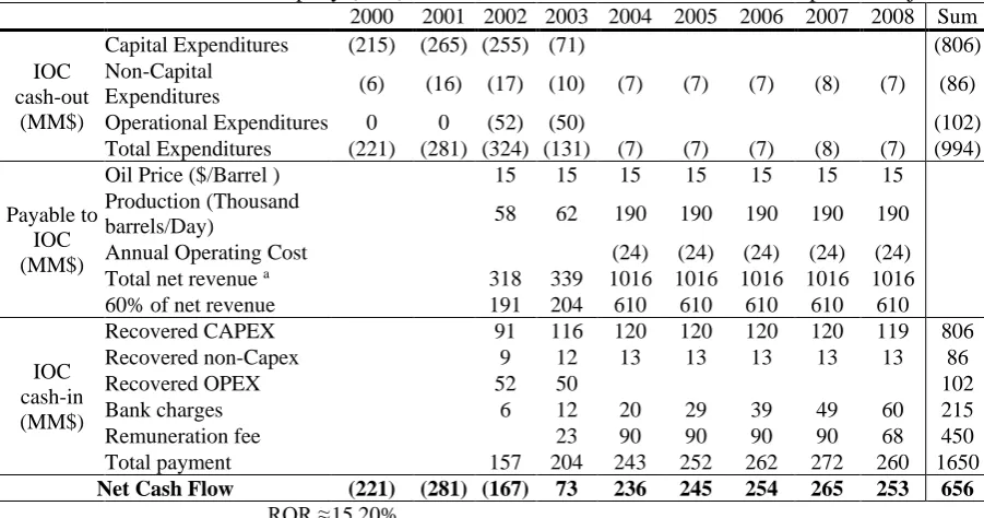
According to Equation (12), as the total expenditures are constant, deferring the costs results in a better NPV. This is due to the very fact that the deferred costs are applied with a larger dominator in the formula, so the company must be very careful during assigning these numbers to cash flow. The original estimated cash flows at the time of contracting is shown in Table 12 and it is evident from the table that IOC’s expected rate of return was 15.20%, about 10% higher than the rate for US treasury bill in that year (1999). According to Table 1, the project cash flow has three major sections: cash out, cash in, and payable net revenue which is the IOC’s share of oil revenues which acts as a controlling element since the installments cannot overstep this amount. It is only activated in period 4, where recoverable amount exceeds the repayable.
Table 1. International oil company (IOC) Investment in Sorous and Norouz Development Project
2000 2001 2002 2003 2004 2005 2006 2007 2008 Sum IOC
cash-out (MM$)
Capital Expenditures (215) (265) (255) (71) (806) Non-Capital
Expenditures (6) (16) (17) (10) (7) (7) (7) (8) (7) (86) Operational Expenditures 0 0 (52) (50) (102) Total Expenditures (221) (281) (324) (131) (7) (7) (7) (8) (7) (994)
Payable to IOC (MM$)
Oil Price ($/Barrel ) 15 15 15 15 15 15 15 Production (Thousand
barrels/Day) 58 62 190 190 190 190 190 Annual Operating Cost (24) (24) (24) (24) (24) Total net revenue a 318 339 1016 1016 1016 1016 1016 60% of net revenue 191 204 610 610 610 610 610
IOC cash-in (MM$)
Recovered CAPEX 91 116 120 120 120 120 119 806 Recovered non-Capex 9 12 13 13 13 13 13 86
Recovered OPEX 52 50 102
Bank charges 6 12 20 29 39 49 60 215 Remuneration fee 23 90 90 90 90 68 450 Total payment 157 204 243 252 262 272 260 1650
Net Cash Flow (221) (281) (167) 73 236 245 254 265 253 656
ROR ≈ 15.20%
a Total net revenue=(oil price ($/Barrel)×Production(Barrels/Day)×365)-annual operating cost
4.3. M-DNPV analysis
The valuation procedure in the M-DNPV starts with risk identification. In reality, this step is usually done by jury of experts or a group decision-making method such as Delphi (Pritchard, 2015). In the current case, the risk origins can be divided into 5 categories including LIBOR, oil price, production, expenditures, and political risks. In what follows, the ways of incorporating these risks into the valuation process are described in detail.
4.3.1. LIBOR risk
All the expenditures are paid with their interest based on London Interbank Offered Rate (LIBOR). As this interest is reflected in the company’s income, any adverse change in LIBOR changes the project profit. To price this risk, following Espinoza and Morris (2013), the Black-Sholes option pricing model is used. In so doing, annual standard deviation of announced rates must be calculated. The 30-days LIBOR rates reported by “Telerate-Page 3750” in 1999 (the year in which valuation is being carried out) are shown in Figure 2. According to this data,
standard deviation of LIBOR percentage changes in the year 1999 was 15.25%; by applying this number to synchronized BS model (exercise price= current price=1, t=1) to calculate the value of a put option using average 10-year long-term government bond rates in 1999 as risk-free rate (5.64%), 𝜂𝑅𝐿𝐼𝐵𝑂𝑅 equals 0.035. By putting this number as risk proxy into Equation (9) and use the output of Equation (7), we can calculate risk premiums related to LIOBR changes. However, to price a proper insurance product, uncertainty coefficient has to be computed. To compute uncertainty coefficients related to LIBOR risk, the variance ratio of LIBOR data series is required. To this aim, the annual average of announced 30-days LIBOR rates for the period between 1987 and 1998 is used to compute autocorrelation coefficients up to 8th order to be
used in Equation (5). The logic behind choosing maximum 8th order autocorrelation coefficient lies in the formula as k is between 1 and t-1, where t is the period at which uncertainty coefficient is calculated. Using Eviews software to calculate kth order autocorrelation coefficient
and plugging them into Equation (5) the results will be as Table 2.
Figure 2. US Dollar 1-month LIBOR rates in 1999 - Telerate Page 3750
Table 2. Computing Uncertainty Coefficients and risk premiums for LIBOR
𝑡 1 2 3 4 5 6 7 8 9
𝑉𝑅
̅̅̅̅(𝑡) 1.000 1.724 2.095 2.158 2.042 1.879 1.732 1.606 1.489
UCt 1.000 1.857 2.507 2.938 3.196 3.358 3.482 3.584 3.661 Θt 0.036 0.066 0.089 0.105 0.114 0.120 0.124 0.128 0.131
Qt 0.494 1.275 2.322 3.497 4.797 6.234 7.871
The variance ratio, 𝑉𝑅̅̅̅̅(𝑡), in Equation 5 is calculated for each future period (t) by the use of autocorrelation coefficients, then by plugging
𝑉𝑅
̅̅̅̅(𝑡) into Equation (6), uncertainty coefficients are computed for each time horizon. The LIBOR risk premiums (Qt), in million dollars, are then calculated with multiplying Θt by the expected interest revenues in each year.
4.3.2. Oil price risk
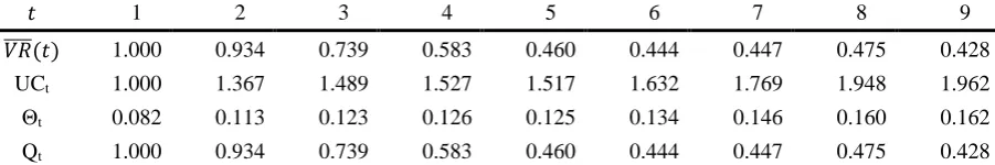
Just like LIBOR, any changes in oil price influences project income through a drop in compensation payment for the expenditures (including capital expenditures, non-capital expenditures, and operational expenditures). The way to deal with this risk is as same as done previously for LIBOR. Here, OPEC’s Annual Statistical Bulletin 1999 is used as empirical data gathered in Figure 3. Following the procedure done for LIBOR, oil price risk proxy (𝜂𝑅𝑜𝑖𝑙) equals 0.0997, and uncertainty coefficients using 1987 to 1999 oil price data are computed in Table 3.
Figure 3. Iran’s heavy crude oil prices (per barrel) in 1999
Jan Feb Mar Apr May Jun Jul Aug Sep Oct Nov Dec Mean 4.979 4.940 4.946 4.924 4.914 5.020 5.180 5.281 5.380 5.410 5.490 6.469
High 5.060 4.963 4.966 4.938 4.944 5.210 5.188 5.371 5.383 5.423 5.608 6.490 Low 4.939 4.935 4.934 4.903 4.900 4.943 5.164 5.202 5.375 5.401 5.400 6.460 4.50
5.00 5.50 6.00 6.50
Jan Feb Mar Apr May Jun Jul Aug Sep Oct Nov Dec Oil prices 9.97 9.54 11.77 14.32 15.05 14.98 17.3 18.96 21.77 21.68 23.26 24.32
In oil price data series, 𝑉𝑅̅̅̅̅(𝑡) < 1 exhibits that the data has a negative serial dependence so its uncertainty coefficients are smaller than LIBOR that has a positive serial dependence. It shows that neglecting serial dependence in long-term and assuming a random walk hypothesis for data series can lead to significant overestimation or underestimation.
Table 3. Computing Uncertainty Coefficients and risk premiums for Oil price
𝑡 1 2 3 4 5 6 7 8 9
𝑉𝑅
̅̅̅̅(𝑡) 1.000 0.934 0.739 0.583 0.460 0.444 0.447 0.475 0.428
UCt 1.000 1.367 1.489 1.527 1.517 1.632 1.769 1.948 1.962 Θt 0.082 0.113 0.123 0.126 0.125 0.134 0.146 0.160 0.162 Qt 1.000 0.934 0.739 0.583 0.460 0.444 0.447 0.475 0.428 The variance ratio in Equation 5 is calculated for each future period (t) by the use of autocorrelation coefficients, then by plugging 𝑉𝑅̅̅̅̅(𝑡) into Equation (6), uncertainty coefficients are computed for each time horizon. The oil price risk premiums (Qt), in million dollars, are then calculated with multiplying Θt by compensation payment for expenditures (CAPEX, non-CAPEX, and PEX) from oil revenues.
4.3.3. Production risk
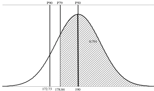
The company may fail to achieve the production target which can affect the remuneration fee. The production rate for the fields is expected to be 190,000 barrels per day, thus if it comes lower than this amount the company may lose money. To account for this risk and to design a synthetic insurance package, it is assumed that the production rate may fluctuate between ±10% of what anticipated with the chance of 90%. In other words, the ratio 𝑝50
𝑝90 equals 1.1, where 𝑝90 and 𝑝50 indicate that the production rate will exceed this amount (i.e 𝑝90 and 𝑝50) 90% and 50% of the time, respectively. With these two parameters (the average production rate and the ratio 𝑝50
𝑝90) a normal distribution can be fitted to production rate. By considering these parameters and assuming a normal distribution, the standard deviation (σ) can be calculated as:
𝑁 (𝑝90−𝑝50
σ ) = 0.1 (13)
where N is the standard cumulative normal distribution and 𝑁−1(0.1) = −1.281, thus σ = 13.477. As the calculations in Table 1 are done based on an average production rate, any rate below this amount is actually a loss and the expected value of loss is represented by the center of gravity of the area to the left of the mean of distribution (i.e. 𝑝50). The described normal distribution for production is plotted in Figure 4. After a typical calculation for the center of gravity, it is located at 178.84 barrels per day which equivalent to 𝑝79 meaning that 79% of times the production rate is greater than this amount and is shown through hatch area in Figure 4. Finally, the synthetic insurance premium for production can be calculated as the difference between the expected production rate (the mean of distribution) and the expected loss (𝑝79). Hence, the normalized insurance premium is:
(190−178.84
190 ) × Pr(𝑝𝑟𝑜𝑑𝑢𝑐𝑡𝑖𝑜𝑛 < 190) = 2.93%.
In M-DNPV methodology, it is important to identify the true source of risks and more importantly where to reflect them. In this case even if production rate be halved, the company can still recover its expenditures but the remuneration fee will fall. Therefore, the annual cost of risk that covers lower production than expected is 2.93% of the expected remuneration fee in each year. As for uncertainty coefficient, since the serial dependence of data is unknown therefore we have:
Figure 4. The normal distribution plot of production rate (in thousands), Mean=190, σ=13.477.
4.3.4. Expenditures risk
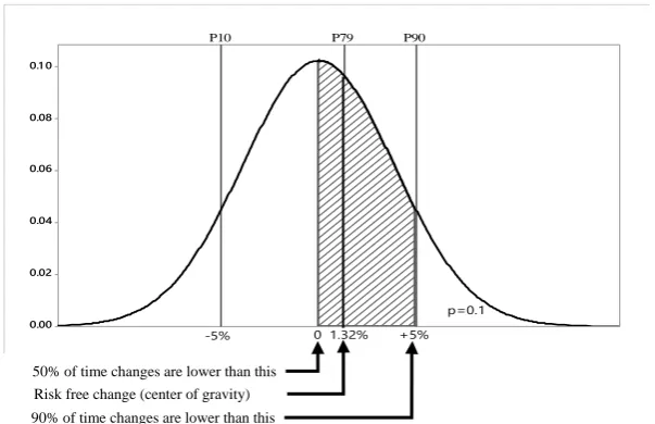
Expenditures risk refers to the cost over-run derived from some technical and/or market reasons. This cost over-run may result in failing to compensate for the project capital expenditures. Following the same procedure done for the production risk and by the use of cost contingencies recommended by Association for the Advancement of Cost Engineering, a normal distribution is fitted to expenditures which is plotted in Figure 5. The expected changes in estimated costs equals zero which is considered as the mean of normal distribution thus anything above this value is considered a loss. Cost contingency for construction is between -5% and +5% of estimated costs. As the nature of data is cost (unlike production in which data was associated with revenues) thus 𝑝50 and 𝑝90 have different definitions and are specified values that costs are lower than 50% and 90% of the time (i.e. 𝑝50= 0 and 𝑝90 = +5%). Skipping the repetitive calculation process, the annual price of risk covering higher expenditures than expected is 1.32% of the estimated annual expenditures (including capital expenditures, non-capital expenditures, and operational expenditures). Due to the unavailability of data series for project expenditures, here US dollar inflation3 is considered to be a proxy for time dependence of costs and the related computations corresponding uncertainty coefficients of expenditures are done through Table 4.
Table 4. Computing Uncertainty Coefficients and risk premiums for Expenditures
𝑡 1 2 3 4 5 6 7 8 9
𝑉𝑅
̅̅̅̅(𝑡) 1.000 0.934 0.739 0.583 0.460 0.444 0.447 0.475 0.428
UCt 1.000 1.367 1.489 1.527 1.517 1.632 1.769 1.948 1.962 Θt 0.082 0.113 0.123 0.126 0.125 0.134 0.146 0.160 0.162 Qt 1.000 0.934 0.739 0.583 0.460 0.444 0.447 0.475 0.428 The variance ratio in Equation 5 is calculated for each future period (t) by the use of autocorrelation coefficients, then by plugging 𝑉𝑅̅̅̅̅(𝑡) into Equation (6), uncertainty coefficients are computed for each time horizon. The expenditures risk premiums (Qt), in million dollars, are then calculated with multiplying Θt by estimated expenditures for each period.
3 Gathered from World Bank
0.791
190 P50
P90 P79
Figure 5. The normal distribution plot of changes in expenditures, Mean=0, σ=3.901 .
4.3.5. Political risk
A company is exposed to political risk in a Foreign Direct Investment (FDI) platform. Political risk refers to situations where host government actions negatively affect the expected return of the international company. There are situations in which host country may fail to comply with its contractual obligations or even refuse to adhere to its binding agreements. During economic crisis or war for instance. The common approach in international businesses to assess political risk is to use country’s sovereign spread which is actually the difference between the yield on a bond issued by a country in US dollars and a US bond of similar maturity. Political risk is then reflected in the valuation by augmenting the discount rate (e.g. (Damodaran, 2012). Given that sovereign spreads are not just influenced by political risk the procedure is questionable. It is recently estimated that using sovereign spreads to proxy political risk leads to overstatement of discount rates by 2-5 percent potentially resulting in remarkable misallocation of international investments (Bekaert, Harvey, Lundblad, and Siegel, 2014). Therefore, we must look for a solution that assesses political risk correctly and its results can be incorporated into cash flows. Bekaert, Harvey, Lundblad, and Siegel (2016) argue that while sovereign spreads are impacted by political risk, they are also influenced by other factors that maybe already included in the valuation which can lead to double counting of risks. To avoid such problematic issues, they propose to use political risk sovereign spreads (PRSS) which is the specific portion of sovereign spread related to political risk. To extract political risk from sovereign spread they regress observed spreads on global factors, local factors, illiquidity index, and political risk ratings of International Country Risk Guide (ICRG). They report the calculated PRSS for each country in the Appendix C of their paper. Then, the reported PRSS can be turned into probability numbers using equation below:
𝑃𝑟𝑜𝑏𝑎𝑏𝑖𝑙𝑖𝑡𝑦 = 𝑃𝑅𝑆𝑆
1+𝑃𝑅𝑆𝑆 (15)
For the case in this paper the method cannot be used directly because Iran has no issued bond in US and consequently has no available sovereign spread. Hence, the available data of other countries is used to find the relation between political risk sovereign spread and ICRG political risk ratings. Therefore, a quadratic cross-sectional regression is run as follows:
𝑃𝑅𝑆𝑆𝑖,𝑡 = 𝑎 𝑃𝑅𝑖,𝑡2 + 𝑏 𝑃𝑅𝑖,𝑡+ 𝑐. (16)
Where 𝑃𝑅𝑖,𝑡denotes political risk rating in time t and country i which is plugged from ICRG ratings. The reason of using a non-linear equation is in the ratio approach used by Beakert et al.
0.1 0
0.08
0.06
0.04
0.02
0.00
0
P90 P79 P10
+5% p=0.1
-5% 1.32%
50% of time changes are lower than this
Risk free change (center of gravity)
(2016). After running the regression powered by an adjusted R-squared exceeding 60% and replacing calculated coefficients, the equation will be:
𝑃𝑅𝑆𝑆𝑖,𝑡 = 0.075𝑃𝑅𝑖,𝑡2 − 17.734 𝑃𝑅𝑖,𝑡+ 1046.923 (17)
by putting 65 as Iran’s 1999 political risk rating (PRiran,1999) into Equation(17), the PRSS will
be 213 bp (100 basis points = 1%) by applying which into Equation(15) the probability of political risk event in Iran equals 2.08%.
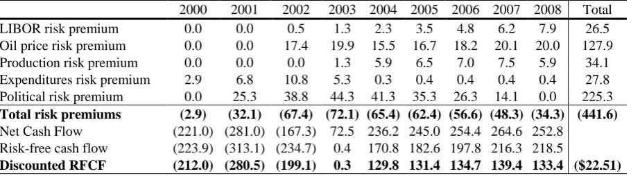
After measuring the political risk event, we have to discuss how it affects the project cash flows. The most threatening aspect of political risk is direct expropriation in which sovereign goes to seize the assets. Furthermore, there are different unfavorable political situations that may lead to the permanent shut down of the project. Under such circumstances, the investor will fail to collect all future expected profits, thus to account for potential of loss, all future cash flows must be discounted to the year in which expected loss is being calculated. The discount rate for this aim should be empty from risk since it must only reflect opportunity cost. The opportunity cost in this case is 5.64%, which is the annual average of long-term 10-year US government bond rate reported by US Department of The Treasury. The calculation of expropriation risk premiums (ERP) which starts from the end of year 2 are done through Table 5 by multiplying discounted remaining revenues in a given year by the probability of political risk and the related uncertainty coefficients. The risk-free cash flow of the project, provided in Table 6, is obtained through applying the synthetic insurance prices calculated in the previous
sections. The calculation done by Equation (11) using 5.64% as the risk-free rate results in a
negative M-DNPV (= -22.51 million dollars). Meaning that the investor must turn down this opportunity or start negotiation for a positive M-DNPV. Based on the traditional methods, to have a positive M-DNPV the investor options are limited to demand a higher remuneration fee or an extension of repayment period.
Table 5. Political risk premiums (million dollars)
Year 2000 2001 2002 2003 2004 2005 2006 2007 2008 Discounted
Revenues ERP
2000 - - - - -
2002 (158.3) 65.0 200.3 196.7 193.4 190.4 172.2 859.7 25.3
2003 68.7 211.6 207.8 204.3 201.1 181.9 1,075.4 38.8
2004 223.6 219.5 215.8 212.4 192.2 1,063.5 44.3
2005 231.9 228.0 224.4 203.0 887.3 41.3
2006 240.8 237.1 214.4 692.4 35.3
2007 250.4 226.5 477.0 26.3
2008 239.3 239.3 14.1
2009 - -
4.4. Final results and discussion
By neglecting uncertainty coefficient and performing typical Decoupled NPV method, the DNPV of the project will be 37.1 MM$, significantly higher than the M-DNPV. Although the
positive DNPV means that project is attractive, as this project was fully repaid by 2010, it is
Table 6. M-DNPV analysis - Risk-free cash flow
2000 2001 2002 2003 2004 2005 2006 2007 2008 Total LIBOR risk premium 0.0 0.0 0.5 1.3 2.3 3.5 4.8 6.2 7.9 26.5 Oil price risk premium 0.0 0.0 17.4 19.9 15.5 16.7 18.2 20.1 20.0 127.9 Production risk premium 0.0 0.0 0.0 1.3 5.9 6.5 7.0 7.5 5.9 34.1 Expenditures risk premium 2.9 6.8 10.8 5.3 0.3 0.4 0.4 0.4 0.4 27.8 Political risk premium 0.0 25.3 38.8 44.3 41.3 35.3 26.3 14.1 0.0 225.3
Total risk premiums (2.9) (32.1) (67.4) (72.1) (65.4) (62.4) (56.6) (48.3) (34.3) (441.6)
Net Cash Flow (221.0) (281.0) (167.3) 72.5 236.2 245.0 254.4 264.6 252.8 Risk-free cash flow (223.9) (313.1) (234.7) 0.4 170.8 182.6 197.8 216.3 218.5
Discounted RFCF (212.0) (280.5) (199.1) 0.3 129.8 131.4 134.7 139.4 133.4 ($22.51)
While by the use of classic methods in decisions regarding whether a project is worth the funding investors are somehow under influence of a Boolean logic (take it or leave it), in the new proposed M-DNPV, after identifying and pricing risks, both parties are able to negotiate the amount and the type of risk that matches their risk appetite to reach an agreement on a feasible risk sharing mechanism. Such agreement has a good chance to be reached through a clear and unbiased view of risky aspects of the project supported by valid risk assessment techniques. If so, it leads to a reduction in risk premium and may make a rejected project economically viable. As a useful contribution of the new method, the risks can be easily prioritized based on their price. This prioritizing can instruct the parties in the negotiation to focus on which risks more. For instance, in the given example foreign investor and the host country (Iran) could agree to equally share the political risk (as the most threatening risk) as a result of which the related premium would reduce to 50% and by this reduction the M-DNPV would be 65 million dollar (87 million higher) concluding a much better project profitability index. Different risk sharing actions can be taken to protect the project cash flow from a fraction of the expected revenues. Without a good and clear risk assessment technique and more importantly without a good method compatible with risky situations, the parties have to rely on heuristic arguments (just like selecting rate of return) rather than a robust numerical reasoning which can lead to a bad agreement. Furthermore, parties must spend a lot of time to reach a mutual definition of a win-win solution which would be finally far away from a no-win situation rooted in using a non-numerical approach.
6. Conclusions
This paper examined and reconciled different debatable factors in project valuation to represent a better easy-to-implement method by combining concepts from tail risk management and capital budgeting. The proposed method is genuinely derived from Certainty Equivalent Method (CEM) and Decoupled Net Present Value (DNPV), and is equipped with new risk management and measurement techniques. The kernel of the method is the synthetic insurance concept used to obtain risk-free cash flows. The risk free cash flows are then discounted using risk-free discount rate. The term “Uncertainty Coefficient” has also been coined to cover the time scaling of risk and to fill the gap between risk and uncertainty in energy megaprojects.
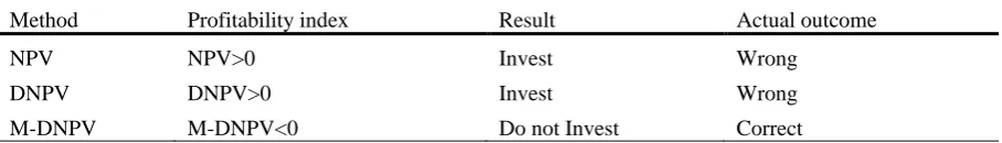
The salient features of the new proposed method are its applicability and simplicity along with its ability to link risk assessment with evaluation using common spreadsheets applications. As the example illustrates, the use of M-DNPV method provides investors with a robust framework to accurately analyze different risk profiles associated with long-lived energy projects, also explained how risk sharing mechanisms can be easily equipped to yield better results. Moreover, the example clearly shows how the new M-DNPV method can be utilized to value difficult-to-evaluate projects without resorting to heuristic arguments for the selection of risk-adjusted rate of return. In addition, it is far obvious that in such high risk projects capital budgeting analysis cannot be reliable unless uncertainty and changing nature of risk are taken into account. Table 7 compares the results of different approaches used in the practical application and it is crystal clear that by considering the disparity between risk, uncertainty, and the time value of money, theoretical concepts of the M-DNPV can close the gaps in existing valuation techniques in long-term megaprojects in energy sector. It also provides investors with a new tool to prioritize risks, leading to ease of decision-making process.
Table 7. Comparing the reliability of different approaches of valuation in predicting profitability of
Soroush and Nowrouz development project
Method Profitability index Result Actual outcome
NPV NPV>0 Invest Wrong
DNPV DNPV>0 Invest Wrong
M-DNPV M-DNPV<0 Do not Invest Correct
This can be particularly useful in energy portfolio management and selecting between heterogeneous projects. It is needless to highlight that the new proposed method has a great flexibility to be used in different energy investments, especially the renewable ones.
Refrences
Baker, R., and Fox, R. (2003). Capital investment appraisal: a new risk premium model. International Transactions in Operational Research, 10(2), 115-126.
Bekaert, G., Harvey, C. R., Lundblad, C. T., and Siegel, S. (2014). Political risk spreads. Journal of International Business Studies, 471–493.
Bekaert, G., Harvey, C. R., Lundblad, C. T., and Siegel, S. (2016). Political risk and international valuation. Journal of Corporate Finance, 1-23.
Bhattacharya, S. (1978). Project Valuation with Mean-Reverting Cash-Flow Streams. Journal of Finance, 1317-1331.
Block , S. (2007). Are real options actually used in the real world? Engineering Economist, 52(3), 255-267. Booker, J. M., and Rossb, T. J. (2011). An evolution of uncertainty assessment and quantification. Scientia
Iranica, 18(3), 669–676.
Carmichael. (2016). Adjustments within discount rates to cater for uncertainty—Guidelines. The Engineering Economist, 1-14. doi:10.1080/0013791X.2016.1245376
Chiara, N., and Garvin, M. J. (2008). Variance models for project financial risk analysis with applications to greenfield BOT highway projects. Construction Management and Economics, 26(9), 925-939.
Chiaroni, D., Chiesa, M., Chiesa, V., Franzò, S., Frattini, F., and Toletti, G. (2016). Introducing a new perspective for the economic evaluation of industrial energy efficiency technologies: An empirical analysis in Italy. Sustainable Energy Technologies and Assessments, 15(Supplement C), 1-10. doi:https://doi.org/10.1016/j.seta.2016.02.004
Damodaran, A. (2012). Investment valuation-tools and techniques for determining the value of any asset (pp. 67). Hoboken-New Jersey: John Wiley and Sons.
Dean, J. (1951). Capital Budgeting. Columbia University Press.
Espinoza, R. (2014). Separating project risk from the time value of money: A step toward integration of risk management and valuation of infrastructure investments. International Journal of Project Management. Espinoza, R., and Morris, J. W. F. (2013). Decoupled NPV: a simple, improved method to value.
Construction Management and Economics.
Fama, E. F. (1977). Risk-Adjusted Discount Rates and Capital Budgeting Under Uncertainty. Journal of Financial Economics, 3-24.
Fisher, I. (1930). The theory of interest: Kelley and Millman.
Fox, R. (2011). A brief critical history of NPV. Paper presented at the British Accounting Association Conference, Blackpool.
Galway, L. A. (2004). Quantitative risk analysis for project management: a critical review. Working Paper No. WR112-RC, RAND Corporation, Santa Monica.
Ghandi, A., and Lawel, C.-Y. C. L. (2015). On the rate of return and risk factors to international oil companies in Iran's Buy-back service contracts.
Ghandi, A., and Lin, C.-Y. C. (2014). Oil and gas service contracts around the world: A review. Energy Strategy Reviews, 63-71.
Halliwell, L. J. (2001). A critique of risk-adjusted discounting. Paper presented at the 32nd International Actuarial Studies in Non-Life Insurance Colloquium, Washington,DC.
Hanafizadeh, P., and Latif, V. (2011). Robust net present value. Mathematical and Computer Modelling, 233-242.
Knight, F. (1921). Risk, Uncertainty, and Profit.
Liou, F. M., and Huang, C. P. (2008). Automated approach to negotiations of BOT contracts with the consideration of project risk. Journal of Construction Engineering and Management Science, 134(1), 18-24.
Lo, A. W., and MacKinlay, A. C. (1988). Stock Market Prices Do Not Follow Random Walks: Evidence from a Simple Specification Test The Review of Financial Studies, 1(1), 41-66.
Mian, M. A. (2011). Project Economics and Decision Analysis, Volume 1. Tulsa, Oklahoma: PennWell Corporation.
Miller, L. T., and Park, C. S. (2002). Decision Making Under Uncertainty—Real Options to the Rescue? The Engineering Economist, 47(2), 105-150.
Myers, S., and Turnbul, S. (1977). Capital Budgeting and the Capital Asset Pricing Model: Good News and Bad news. Journal of Finance, 321-333.
PMBOK. (2013). PMBOK Guide – Fifth Edition (pp. 309-354). Pennsylvania: Project Management Institute, Inc.
Pritchard, C. L. (2015). Risk Management-Concepts and Guidance,Fifth Edition-PMP, PMI-RMP, EVP: Taylor and Francis Group.
Robichek, A., and Myers, S. (1966 ). Conceptual problems in the use of risk-adjusted discount rates. The Journal of Finance, 727–730.
Schmalensee, R. (1981). Risk and Return on Long-Lived Tangible Asset. Jownal of Financial Economic, 185-205.
SHANA (2010). Share of Soroush and Norouz in Increasing Irans Oil Output [Press release]. Retrieved from http://www.shana.ir/en/newsagency/59208/Share-of-Soroush-Norouz-in-Increasing-Irans-Oil-Output Sharpe, W. F. (1964). Capital asset prices: A theory fo market equilibrium under conditions of risk. The
Journal of Finance, 19(3), 425-442.
Shimbar, A., and Ebrahimi, S. B. (2017). The application of DNPV to unlock foreign direct investment in waste-to-energy in developing countries. Energy, 132, 186-193.
Shiravi, A., and Ebrahimi, S. N. (2006). Exploration and development of Iran’s oilfields through buyback. Natural Resources, 199-206.
Shiravi, A., and Majd, F. A. (2015). Foreign investment in Iran’s upstream oil and gas operations: a legal perspective. The Journal of World Energy Law and Business.
Van Groenendaal, W. J. H., and Mazraati, M. (2006). A critical review of Iran’s buyback contracts. Energy Policy, 3709-3718.
Wang, J.-N., Yeh, J.-H., and Cheng, N. Y.-P. (2011). How accurate is the square-root-of-time rule in scaling tail risk: A global study. Journal of Banking and Finance, 35(5), 1158-1169.
Ye, S., and Tiong, R. L. (2000). NPV-at-risk method in infrastructure project investment evaluation. Journal of Construction Engineering and Management, 126(3), 227-233.