Modeling of Influence of Climate Change Character on
the Territory of the Cryolithozone on the Value of
Risks for the Road Network
https://doi.org/10.3991/ijoe.v16i07.14557
Yu.V. Trofimenko (*), A.N. Yakubovich, I.A. Yakubovich, E.V. Shashina Moscow Automobile and Road Construction State Technical University (MADI),
Moscow, Russia [email protected]
Abstract—The level of climate risks is proposed to be estimated by the amount of thawing soil settlement in the formation of automobile roads, corre-sponding to the accepted scenario of the climate change. An updated algorithm is presented, according to which the average risk assessment for a 4-year period is divided into a risk assessment for individual years. Calculations performed for the climatic conditions of Yakutsk and Urengoy establish a significant depend-ence of the predicted risk on the warming pattern. The level of risk predicted when the average annual air temperature increases by 2 degrees is estimated as average (up to 526 points on a 1000-point scale). The most appropriate method of reducing this risk is to perform timely repairs to bring the road to the standard technical and operational condition without the use of special technologies for regulating the temperature regime of soil.
Keywords—Climate change, Road Network, Cryolithozone, Modeling, Soil Thawing, Climate Risks.
1
Introduction
1.1 Review of literature
the upper layer of permafrost) leads to the appearance of additional settlements of the thawing soil and deformation of road structures, which causes deterioration of their technical and operational properties up to destruction. In particular, numerous chaoti-cally located road surface subsidence’s naturally lead to the maximum possible traffic flow speed decrease and the road capacity reduction [4]. Possible empirical methods for evaluating the road surface condition parameters, in particular, its width, are de-scribed in [5]. The use of a multi-purpose radio-controlled car for this purpose is shown in [6].
Among the studies devoted to the influence of natural and climatic conditions on the technical and operational state of the road network, the following can be distinguished. In [7] it is shown that the express defect of the road slope (as a result of its erosion by the water flow of the increased intensity) leads to the accelerated pavement and road cross section damage; the road cross section resistance level to such external influence depends on the soil type and the slope angle. A new method for estimating seismic risk for transport networks with bridge structures using probabilistic seismic hazard analysis (seismic risk assessment based on the theorem of total probability) is given in [8]. The survival analysis of light cellular concrete used as part of the subgrade is performed in [9]. The method for survival assessing includes building a multi-level model for evalu-ating factors that affect the concrete functional performance (analytical hierarchy), building a membership function for each factor, and obtaining the final complex mem-bership function for a parameter that quantitatively describes the survival (fuzzy inte-gral assessment). In [10] a list of climatic and weather factors is formed, that have the most significant impact on the technical and operational condition of the road; and the structure of information-measuring system is proposed that can fix parameters values reflecting these factors in real time, and can forecast the technical and operational road condition on the basis of constantly updated data.
Quantitative forecasting of the subgrade settlement, taking into account the proba-bilistic nature of the factors affecting it, is performed in [11]. To overcome the weak-nesses and limitations of purely probabilistic and purely deterministic models, a com-bined forecasting model is proposed and numerically implemented, based on an im-proved analysis of set pairs, and taking into account both stochastic and deterministic impacts on the subgrade soil. As a result, it is possible to quantify the amount of fore-casted settlement at different levels of the probability of not exceeding this value. In [12], the development process of loess soil settlement is described quantitatively: its increase over time, starting from the moment of the first subgrade load application.
It should be noted that there are many methods used to forecast the soil settlement amount at the base of engineering constructions, and to provide a sufficiently high re-sults accuracy. Subgrade settlement forecasting based on the regression of the reference vector of least squares and the quantum evolutionary algorithm is performed in [13]. A simplified method for settlement forecasting of pivot rings on reinforced cohesionless soils is given in [14].
as compared to that occurs in the climate before the warming beginning). Climate changes are described by a spasmodic increase in the average annual air temperature; as these changes have the probabilistic nature, warming is considered a normally dis-tributed random variable with an average value of +2 °C and is described by a sample of several realizations. For each random variable realizations the expected additional soil settlement at the subgrade is determined and the climate risk is assessed; the final risk value is the settlement weighted average for all the considered realizations.
The forecast values of climate risk obtained in [15] are averaged over a sufficiently long period during which an increase in air temperature is simulated, and the realization order in the sample is not taken into account. Accordingly, the purpose of this work is to analyze in more detail the risks distribution within this period, and to obtain climate risk estimates for the most unfavorable dynamics of temperature changes, described using a sequence of random variable realizations that characterize the increase in the average annual air temperature for individual years of the simulated period.
1.2 Climate risk prediction technique
The main climatic parameters that affect the road network functionality decrease as a result of forecasted climate changes are the air temperature t, C, and the wind speed in the atmospheric boundary layer v, m/s. The quantitative values of these parameters are modeled at a pitch of Δτ for one full average year, the duration of which is assumed to be 365 days. Then, with the same pitch Δτ, the heat exchange is modeled between atmospheric air and soil (the first type), and between individual fragments of the soil mass formed by the road cross section and the formation soil (the second type). Heat transfer of the first type is described by the empirical dependence of Matsumura:
𝑄!= 18𝑣",$%&&𝑡'− 𝑡()𝑆(𝛥𝜏, (1)
where Q1 – the heat energy (J), v – the mean wind speed for the period Δτ (m/s);
ta and tg – the average temperature of atmospheric air and ground surface, respectively (°C); Sg – square of design element of soil mass in contact with atmospheric air (m2).
The values of Q1 > 0 correspond to the heat flow into the soil, where the second type heat exchange models temperature dynamics in the road cross section and its formation. Then the modeled soil mass is divided into individual elements and the heat exchange of the second type between them is described by the formula:
𝑄)=*!),+*#"(𝑡-− 𝑡.)𝛿/𝛿0𝛥𝜏, (2)
where λA and λB – the temperature-dependent coefficients of soil thermal conduction for the contiguous design elements A and B (W/(m∙°C)); δx, δy, δz – the designed soil elements dimensions along the x, y, and z axes (m); tA and tB – the average temperature of the design elements A and B, respectively (°C).
(during the one year) thawing depth hmax (corresponding to the depth of penetration of the temperature isoline t = tbf into the soil, where the soil freezing temperature tbf de-pends on soil type and humidity). Thus, the maximum thawing depth of the formation soil can be represented as:
ℎ1'2= 𝑀(𝑻, 𝑽, 𝑮), (3)
where M – a generalized transformation operator (including, among others, a com-putational procedure for modeling the temperature dynamics of the formation soil); T – an array of atmospheric air temperature values throughout the year; V – an array of wind speed values; G – a set of geometric, physicomechanical, and thermophysical soil parameters.
The magnitude of the section or road network functionality loss risk expected when climate changes occur is considered to depend on the amount of excess soil thawing in the road formation, and on the additional settlement Δm caused by this thawing in the soil mass. To quantify Δm, two climate states are considered: the basic one, character-ized by averaged values of T and V for the period 1960-1990, and the modified one, in which all values of atmospheric air temperatures are assumed to be increased by the same value of n (°C), resulting in an array of temperatures T(n).
The base climate corresponds to the design and construction period of most of the currently operated highways in the cryolithozone of Russia; the changed climate re-flects scenario assumptions about the road network operating conditions for the period up to 2030. The value of excess thawing during climate warming at n °C is defined as:
𝛥ℎ(4)= 𝑀&𝑻(4), 𝑽, 𝑮) − 𝑀(𝑻, 𝑽, 𝑮). (4)
After that, taking into account the physicomechanical parameters of the soil, an ad-ditional settlement Δm(n) in the thawed soil layer with a thickness of Δh(n) is calculated.
The period during which additional thawing soil settlement is simulated and associ-ated climate risks are determined consists of 4 consecutive years. The parameter n is considered a random normally distributed value, with an average value of nmed = +2 °C and a standard deviation of σ=0.85 in order to take into account the variability of climate conditions for individual years. The climate warming is thus described by a sequence of values {n1...n4}, reflecting the atmospheric air temperature increase (compared to the base climate) for individual years of the modeled period.
The selection {n1...n4} corresponding to the accepted values of nmed and σ is deter-mined in sequence (see Fig. 1):
1.The range of possible values of n is divided into 4 sections with equal probability of getting the random variable realization within each of the sections; adjacent bound-aries are determined from the conditions F(n) = 0.25, F(n) = 0.5 and F(n) = 0.75, where F(n) is a function of the normal distribution;
Fig. 1. The air warming value n1–n4 in individual years of the 4-year period under review
The resulting sample of 4 realizations of n, arranged in ascending order, has the form {n1=0.86; n2=1.686; n3=2,316; n4=3,142} (values in C); the average value and the standard deviation of the sample coincide with nmed and σ. At the same time, there may be other implementations sequences in the sample that preserve the specified values of
nmed and σ; there are 24 different sequences in total. Each sequence of ni values reflects a particular variant of the atmospheric temperature dynamics over a 4-year period and, accordingly, one of the possible variations in climate risks during this period. To iden-tify the most dangerous variant with the highest risks, all 24 ni sequences are consid-ered, and for each of them, risks are quantified by three indicators.
The first indicator R1,i reflects the risks expected in the i-th year of the period, and determined directly from the results of modeling additional formation soil settlement
𝛥𝑚6, expressed in cm:
𝑅!,6= 100𝛥𝑚6. (5)
The second indicator R2 reflects the weight-average risk across all years of the period under review; considering the same probability for each of the implementations of ni and hence the same probability for all values of Δmi, the value of average risk is:
𝑅)= 25 ∑768!𝛥𝑚6. (6)
The third risk indicator R3,i is determined by the value Δmi gradient: the specific settlement is calculated (corresponding to an increase in air temperature by +1 °C), which increases by the value of the average warming nmed:
𝑅9,6= 200:14$
$ . (7)
The R2 indicator reflects the most conservative estimation of the climate risk (lower estimate). The maximum value of R3,i for all years of the period, on the contrary, can be considered as the most pessimistic risk estimation (upper assessment). The indicator
2
Results and Discussion
2.1 Numerical simulation results
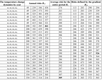
Quantitative risk estimations performed for Yakutsk climatic conditions are shown in the Table 1, the values highlighted in the table correspond to the highest forecasted risk estimates for each of the three indicators R1, R2, and R3. The road body (soil for-mation) height was assumed to be 2 m, the width at the top was 10 m, the formation soil was clay, with high humidity.
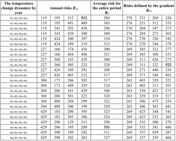
The forecast risks values for the road network (sections) in the Urengoy climate are shown in the Table 2, the geometric dimensions and physicomechanical parameters of the soil mass were assumed to be the same as for Yakutsk.
When performing all calculations, the modelling interval Δτ was assumed to be 1800 s; the geometric dimensions of the soil mass designed element were δx = δy = δz = 0.1 m. Reducing the values of these modelling parameters did not lead to a significant change in the numerical results thus, the accuracy of the values in the tables 1 and 2 can be considered guaranteed.
Table 1. Forecast risks of the road network functionality decrease when the climate warms by 2 °C in the climatic conditions of Yakutsk
The temperature change
dynamics by year Annual risks R1,i Average risk for the entire period R
2
Risks defined by the gradient
R3,i
n1-n2-n3-n4 49 239 346 458 274 113 283 298 294
n1-n2-n4-n3 49 239 373 393 263 113 283 238 339
n1-n3-n2-n4 49 325 301 458 283 113 281 357 292
n1-n3-n4-n2 49 325 381 327 272 113 281 247 388
n1-n4-n2-n3 49 442 312 357 283 113 264 371 308
n1-n4-n3-n2 49 415 366 321 288 113 264 316 380
n2-n1-n3-n4 208 182 285 461 284 246 423 246 293
n2-n1-n4-n3 208 182 439 390 305 246 423 279 337
n2-n3-n1-n4 208 335 213 452 302 246 289 496 288
n2-n3-n4-n1 208 335 456 227 306 246 289 290 521
n2-n4-n1-n3 208 361 159 354 271 246 230 369 306
n2-n4-n3-n1 208 361 357 163 272 246 230 308 378
n3-n1-n2-n4 241 192 289 396 280 208 446 343 252
n3-n1-n4-n2 241 192 442 250 281 208 446 281 297
n3-n2-n1-n4 241 241 210 451 286 208 286 489 287
n3-n2-n4-n1 241 241 452 226 290 208 286 287 526
n3-n4-n1-n2 241 439 163 307 288 208 280 379 364
n3-n4-n2-n1 241 439 244 217 286 208 280 290 505
n4-n1-n2-n3 354 203 294 365 304 226 473 349 316
n4-n1-n3-n2 354 203 294 317 292 226 473 254 376
n4-n2-n1-n3 354 298 144 353 287 226 354 335 305
n4-n2-n3-n1 354 298 352 158 291 226 354 304 367
n4-n3-n1-n2 354 351 219 305 307 226 303 510 362
2.2 Discussion
For all the considered variants of atmospheric temperature dynamics, high risk var-iability is forecasted for individual years of the 4-year period (indicators R1 and R3). According to the indicator R1, this variability is slightly higher in Yakutsk conditions (the maximum change in risk over 4 years is 409 units). In Urengoy conditions, the R1 risk value is also high (393 units). Risk estimates based on the gradient of settlement values R3 have slightly less variability within the simulated period (the largest change over 4 years of the R3 indicator is 318 units for Yakutsk and 254 units for Urengoy).
Table 2. Forecast risks of the road sections functionality decrease when the climate warms by 2 C in the climatic conditions of Urengoy
The temperature change dynamics by
year
Annual risks R1,i
Average risk for the entire period
R2
Risks defined by the gradient
R3,i
n1-n2-n3-n4 119 195 312 512 284 276 231 269 326
n1-n2-n4-n3 119 195 491 409 303 276 231 312 353
n1-n3-n2-n4 119 343 293 430 296 276 284 347 273
n1-n3-n4-n2 119 343 429 308 300 276 284 273 365
n1-n4-n2-n3 119 424 300 397 310 276 270 356 343
n1-n4-n3-n2 119 424 399 319 315 276 270 344 378
n2-n1-n3-n4 227 166 374 436 300 269 385 323 277
n2-n1-n4-n3 227 166 484 408 321 269 385 308 353
n2-n3-n1-n4 227 360 183 429 300 269 311 426 273
n2-n3-n4-n1 227 360 505 225 329 269 311 322 522
n2-n4-n1-n3 227 426 189 391 308 269 271 440 338
n2-n4-n3-n1 227 426 403 212 317 269 271 348 492
n3-n1-n2-n4 304 173 286 505 317 263 403 339 321
n3-n1-n4-n2 304 173 489 329 324 263 403 311 391
n3-n2-n1-n4 304 286 181 429 300 263 339 421 273
n3-n2-n4-n1 304 286 501 223 328 263 339 319 517
n3-n4-n1-n2 304 480 204 299 322 263 306 475 354
n3-n4-n2-n1 304 480 306 190 320 263 306 363 441
n4-n1-n2-n3 429 183 290 395 323 269 425 344 341
n4-n1-n3-n2 429 183 385 306 324 269 425 332 363
n4-n2-n1-n3 429 296 129 313 290 269 352 300 270
n4-n2-n3-n1 429 296 395 209 331 269 352 341 486
n4-n3-n1-n2 429 390 189 242 311 269 337 439 287
n4-n3-n2-n1 429 390 302 201 327 269 337 359 466
The spread of risk values obtained taking into account possible differences in the dynamics of the temperature regime of atmospheric air in the territory of Yakutsk is: for the indicator R1 – 30% (R1,min=354, R1,max=461), for the indicator R2 – 17% (R2,min=263, R2,max=309), for the indicator R3 – 77% (R3,min=298, R3,max=526). In Uren-goy climatic conditions, the possible values spread is: for R1 – 21% (R1,min=424, R1,max=512), for R2 – 17% (R2,min=284, R2,max=331), for R3 – 60% (R3,min=326, R3,max=522).
forecasted on the basis of averaged temperature parameters over the entire period. Only an analysis of all possible variations of temperature changes in the territory can reliably identify the maximum possible risk. It is also necessary to note the impact of the par-ticular territory climatic features on the risk values, which is most noticeable in relation to R1.
The maximum forecasted climate risk level obtained from numerical simulation is
R3=526 units and corresponds to the climate conditions of Yakutsk; in relation to the climatic features of Urengoy, the upper limit of the expected risk R3 is at the level of 522 units. The qualitative interpretation of the risk values is described in [13]; according to it, the maximum risk, which means the complete functionality loss of the road sec-tion, corresponds to the value R=1000. The range of values 301≤R<600, to which the
R3 values belong for both examples considered, corresponds to the upper sublevel of the average risk. The lower risk estimate, based on weighted average values over a 4-year period, is R2=331 for Urengoy and R2=309 for Yakutsk; these values also allow to classify the risk as the average level one (lower sublevel).
3
Conclusion
The atmospheric air temperature dynamics influence on the risks level for roads sec-tions (network) in the cryolithozone is significant and causes a change in the forecasted risk value from 17% to 77%. Identification of the most unfavorable temperature dy-namics, at which the maximum road malfunction risk is forecasted, is an essential con-dition for obtaining reliable quantitative estimates of climate risks.
The risk level forecasted for road sections (network) in the area of Yakutsk and Uren-goy, with the increase in the average annual air temperature as a result of climate warm-ing up to +2 °C and the most dangerous nature of climate change, is estimated as aver-age. This risk level involves constant monitoring of the road surface current state and timely repair works to eliminate defects that occur due to excessive soil formation thaw-ing and settlement. The use of technologies for adaptation of road facilities that regulate the soil temperature regime (thermal insulation coatings, seasonal cooling devices) and prevent the occurrence of excess soil settlement is not mandatory for average risks. However, the final decision on the application of engineering measures to adapt specific roads sections in the regions under consideration should be made on the basis of detailed technical and economic calculations.
4
References
[1]Driga, A.M., Drigas, A.S. “Climate Change 101: How Everyday Activities Contribute to the Ever-Growing Issue”, International Journal of Recent Contributions from Engineering, Sci-ence & IT, vol. 7(1), pp. 22-31, 2019. https://doi.org/10.3991/ijes.v7i1.10031
[2]Gruza, G.V. and et. “Features of the temperature regime at the surface of the globe in 2018”,
[3]Anisimov, O., Kokorev, E., Zhiltcova, Y. “Arctic ecosystems and their services under chang-ing climate: predictive-modelchang-ing assessment”, Geographical Review, vol. 107(1), pp. 108-124, 2017 https://doi.org/10.1111/j.1931-0846.2016.12199.x
[4]Yakubovich, A.N., Trofimenko, Yu.V., Yakubovich, I.A., Shashina, E.V. “A forecast model for a road network’s section traffic capacity assessment on a territory of the cryolithozone in conditions of the climate change”, Periodicals of Engineering and Natural Sciences, vol. 7(1), pp. 275-280, 2019 https://doi.org/10.21533/pen.v7i1.380
[5]Nasution, S.M., Husni, E., Kuspriyanto, Yusuf, R., Mulyawan, R. “Road Information Col-lector Using Smartphone for Measuring Road Width Based on Object and Lane Detection”,
International Journal of Interactive Mobile Technologies, vol. 14(2), pp. 42-61, 2020
https://doi.org/10.3991/ijim.v14i02.11530
[6]Mahbub, M. “Design of a Multipurpose Radio Controlled Surveillance Vehicle to Monitor Risky Areas”, International Journal of Recent Contributions from Engineering, Science & IT, vol. 7(2), pp. 7-29, 2019 https://doi.org/10.3991/ijes.v7i2.10380
[7]Ye, T., Xie, Q., Wang, Y., An, Y., Jin, J. “Analog modeling of sand slope stability with different precipitation conditions”, Journal of Modern Transportation, vol. 26(3), pp. 200-208, 2018 https://doi.org/10.1007/s40534-018-0163-0
[8]Tak, H.-Y., Suh, W., Lee, Y.-J. “System-level seismic risk assessment of bridge transporta-tion networks employing probabilistic seismic hazard analysis”, Mathematical Problems in Engineering, vol. 2019, August, 2019. [Online serial]. Available: https://www.hindawi.com /journals/mpe/contents/year/2019/ [Accessed Apr.1, 2020] https://doi.org/10.1155/2019/ 6503616
[9]Liu, X., Ni, Ch., Zhang, L., Sheng, K., Hong, B. “Durability assessment of lightweight cel-lular concrete in subgrade by the method of analytic hierarchy process combined with fuzzy comprehensive evaluation”, Mathematical Problems in Engineering, vol. 2019, August, 2019.[Online serial].Available:https://www.hindawi.com/journals/mpe/contents/year/2019/
[Accessed Apr. 1, 2020] https://doi.org/10.1155/2019/4915870
[10]Yakubovich, A.N., Yakubovich, I.A., Trofimenko, Yu.V., Shashina, E.V. “Intelligent man-agement system of the automobile road’s technical and operational condition in the cryo-lithozone”, in Proc. Systems of Signals Generating and Processing in the Field of on Board Communications, SOSG 2019’03 2019 https://doi.org/10.1109/sosg.2019.8706742
[11]Li, Y., Leng, W., Nie, R., Mei, H., Zhou, S., Dong, J. “A combined prediction model for subgrade settlement based on improved set pair analysis”, Mathematical Problems in Engi-neering, vol. 2019, August, 2019. [Online serial]. Available: https://www.hindawi.com/ journals/mpe/contents/year/2019/ [Accessed Apr. 1, 2020] https://doi.org/10.1155/2019/10 64246
[12]Ge, M., Li, N., Zhang, W., Zheng, J., Zhu, C. “Settlement behavior and inverse prediction of post-construction settlement of high filled loess embankment”, Chinese Journal of Rock Mechanics and Engineering, vol. 36(3), pp. 745–753, 2017
[13]Gao, H., Song, Q.-C., Huang, J. “Subgrade settlement prediction based on least square sup-port vector regession and real-coded quantum evolutionary algorithm”, International Jour-nal of Grid and Distributed Computing, vol. 9(7), pp. 83–90, 2016 https://doi.org/10.14257/ ijgdc.2016.9.7.09
[14]Tafreshi, S.N.M., Shaghaghi, T., Mehrjardi, G.T., Dawson, A.R., Ghadrdan, M. “A simpli-fied method for predicting the settlement of circular footings on multi-layered geocell-rein-forced non-cohesive soils”, Geotextiles and Geomembranes, vol. 43(4), pp. 332–344, 2015
https://doi.org/10.1016/j.geotexmem.2015.04.006
permafrost regions”, Transportation research procedia, vol. 36, pp. 810-816, 2018.
https://doi.org/10.1016/j.trpro.2018.12.076
5
Authors
Yury Vasilievich Trofimenko is the head of the Technosphere Safety Chair of Mos-cow Automobile and Road Construction State Technical University (MADI), Lenin-gradsky avenue, 64, Moscow, Russia, 125319.E-mail: [email protected]
Anatoly Nikolaevich Yakubovich is a full professor of the Operation and Servicing of Motor Vehicles Chair of Moscow Automobile and Road Construction State Tech-nical University (MADI), Leningradsky Avenue, 64, Moscow, Russia, 125319.
Irina Anatolievna Yakubovich is a full professor of the Operation and Servicing of Motor Vehicles Chair of Moscow Automobile and Road Construction State Technical University (MADI), Leningradsky Avenue, 64, Moscow, Russia, 125319.
Elena Vladimirovna Shashina is an assistant professor of the Technosphere Safety Chair of Moscow Automobile and Road Construction State Technical University (MADI), Leningradsky Avenue, 64, Moscow, Russia, 125319.