Modeling the potential impact of climate change in northern Mexico using two
environmental indicators
A. LÓPEZ SANTOS
Unidad Regional Universitaria de Zonas Áridas, Universidad Autónoma Chapingo, Apartado Postal 8, 35230 Bermejillo, Durango, México
Miembro de la Red Temática del Agua del CONACyT
Corresponding author; e-mail: [email protected]
J. PINTO ESPINOZA
Instituto Tecnológico de Durango, Blvd. Felipe Pescador 1830 Ote., Col. Nueva Vizcaya, 34080 Durango, Durango, México
E. M. RAMÍREZ LÓPEZ
Universidad Autónoma de Aguascalientes, Av. Universidad 940, Ciudad Universitaria, 20131 Aguascalientes, Aguascalientes, México
M. A. MARTÍNEZ PRADO
Instituto Tecnológico de Durango, Blvd. Felipe Pescador 1830 Ote., Col. Nueva Vizcaya, 34080 Durango, Durango, México
Received June 4, 2012; accepted May 28, 2013
RESUMEN
La modelación de impactos locales, caracterizados por deterioro de los recursos naturales –especialmente agua y suelo– ante los efectos globales del cambio climático, se ha convertido en una poderosa herramienta en la búsqueda de medidas de mitigación y adaptación. Los objetivos de la presente investigación fueron: 1) evaluar mediante procesos de modelación el impacto potencial del cambio climático para el periodo 2010-2039 y 2) advertir sobre riesgos futuros a partir de la identificación de forzantes radiativos locales o áreas críticas, considerando el índice de aridez (IA) y erosión laminar del suelo causada por el viento (ELV) como dos indicadores de calidad ambiental. Se usaron técnicas de evaluación de los recursos naturales emplea-das por el Instituto Nacional de Ecología y Cambio Climático (INECC) para los estudios de ordenamiento ecológico territorial. Los insumos empleados comprenden información climática actual y futura, cubiertas de suelos y propiedades edáficas asociadas al municipio de Gómez Palacio, Durango, México (25.886º N y 103.476º W). Los cálculos realizados a partir de las anomalías para los promedios anuales de precipitación y temperatura indican que el territorio municipal en el escenario A2 podría tener un impacto promedio de 63% causado por la ELV, en tanto que el IA probablemente cambie su promedio histórico de 9.3 a 8.7; se estima que el impacto promedio sobre este índice en el futuro será de 0.53 ± 0.2.
ABSTRACT
Evaluation techniques for natural resources, similar to those applied by the Instituto Nacional de Ecología y Cambio Climático (National Institute of Ecology and Climate Change) were used for studies of ecological land use. The inputs include climate information (current and future), soil cover and edaphic properties related to the municipality of Gómez Palacio, Durango, Mexico (25.886º N, 103.476º W). According to calculations estimated from the anomalies for the mean annual rainfall and mean annual temperature, in a future climate change scenario, an average impact of approximately 63% would be caused by LWE, and the AI would change from its historical value of 9.3 to 8.7. It is estimated that the average impact on the AI in the future will be 0.53 ± 0.2.
Keywords: Climate scenarios, modeling, ecological zoning.
1. Introduction
In less than a decade, modeling climate processes to assess the deterioration of natural resources has become a powerful tool for determining trends, es-pecially for water and soil (Yu, 2003; Rose, 2005; van Roosmalen et al., 2011). For example, van Roosmalen et al. (2011) used a model to determine future changes in the recharge of aquifers in a small (5459 km2) hydrological basin in Denmark. They
employed a downscaling method with a resolution of 12 km2 from a regional climatic model (RCM)
with a resolution of 40 km2 identified as HIRHAM4.
That model was then nested into the General Climat-ic Model (GCM) developed by the Hadley Centre.
Recent studies warn about climate changes, partic-ularly alterations in precipitation and temperature vari-ables (Rivera et al., 2007; García-Páez and Cruz-Me-dina 2009). For example, Magaña et al. (2003) and Magaña (2010) argue that under a scenario of global warming, the El Niño/Southern Oscillation (ENSO) cycle could be more frequent and intense, leading to longer drought periods at 25º N latitude, where the state of Durango is located.
These predictions are especially relevant in light of the increasing vulnerability of physical-biotic and socio-economic systems, particularly in the produc-tion of staple crops such as maize in Mexico (Monter-roso et al., 2011). Therefore, there is an urgent need to develop techniques that not only consider future climatic trends (PNUD, 2005) but also that match the information available to effectively assess the probability of local impacts. Such information can strengthen adaptation measures to climate change (SEMARNAT-INE, 2009).
Consequently, the objectives of this research were: (1) to model the potential impact of climate change for the period 2010-2039, and (2) to offer advice about future risks based on local radiative forcing or
critical areas and taking into account two indicators of environmental quality, the aridity index (AI) and soil erosion.
2. Methodology
2.1 Study area, characteristics and location
Gómez Palacio is one of the 39 municipalities of the state of Durango. It has an area of 842.32 km2,
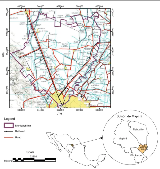
and it is located (25.886 ºN, 103.476 ºW) in a geo-graphical-ecological region known as the Bolsón de Mapimí. This region presents a climate gradient from south to north, ranging from dry (BSohw) to very dry (BWhw). The annual average temperature varies from 20 to 24 ºC, and the mean annual rain-fall is approximately 200 mm (García, 2003). One of its salient characteristics is that approximately 60% of the territory is used for agriculture with irrigation, as is favored by its topography (slope < 1%); the remaining 40% corresponds to urban and rural (Fig. 1).
2.2 Study baseline and indicators of environmental quality (IQA)
The baseline or reference for this study were the con-ditions of 2010, which serve as a basis for comparison to assess the impact of climate change on a 30-year (2010-2039) time horizon. The environmental char-acteristics chosen as indicators were the laminar wind erosion (LWE) and AI, the first as the loss of soil due to the wind action on the soil surface, and the second as drought stress. Each is directly correlated with the changes under future scenarios for temperature and rainfall, as described by Magaña et al. (2012) for the northeast of Mexico.
2.3 IQA modeling and input data
indica-tor, the loss of soil in t ha–1 yr–1 was estimated based
on the methodology proposed by INE (1998) for studies of ecological-use zoning, and (2) AI was de-termined by the De Martonne’s aridity index, which has been used by Mercado-Mancera et al. (2010) as an estimator of the aridity and desertification in arid land in northwestern Mexico.
The input for the baseline year modeling was the historical data set of weather from the Servicio Meteorológico Nacional (SMN, National Weather
Service), as well as measurements related to the bi-otic physical environment such as topography, soil and vegetation. Meanwhile, to assess the potential impact on the IQA by future scenarios (2010-2039), projections (metadata) for regional climate change of Mexico were downloaded (INE-SEMARNAT, 2011). These data were generated by downscaling the results of the global circulation models (GCM) used in the Fourth Assessment Report of the IPCC in 2007 (IPCC, 2008).
636000
636000
644000
644000
652000
652000
660000
660000
668000
668000
2832000 283200
0
2840000 2840000
Tlahualilo
Mapimí
Lerdo Palacio
2864000
Bolsón de Mapimí
Gómez
Scale 22800 Meters
Municipal limit
UTM
UT
M
Railroad
Road Legend
2856000
2864000
2856000
284800
0
284800
0
2.4 Meaning and process for determining LWE The LWE as an environmental quality index rep-resents the magnitude (t ha–1 yr–1) of soil loss by wind,
which theoretically is incorporated as an additional burden at different heights in the atmosphere. In the lower layer, the air carrying soil has direct effects on human health because it is the layer of air that people breathe. Such impacts can reach many kilometers from where it is produced, affecting both rural and urban areas.
Calculating the baseline LWE (for 2010) began with the determination of the dominant environmen-tal factors in erosion, the action of water or wind. The values depend on indices related to edaphic properties (CATEX, Spanish acronym), use of soil (CAUSO, Spanish acronym), susceptibility of soil to erosion (CAERO, Spanish acronym) and topo-graphical conditions (CATOP, Spanish acronym), which apply according to the predominant process in the erosion.
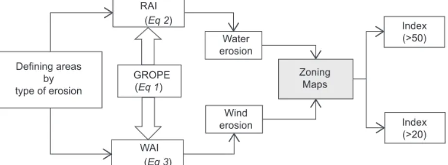
The basis for the calculation of the erosion rates is in both cases (water or wind) related to the avail-ability of humidity as a result of the presence of rain > 10 mm. Therefore, the mean annual rainfall (MAR) was determined to estimate the rain aggressiveness index (RAI) and wind aggressiveness index (WAI). Both indices depend on MAR, which determines the growth period (GROPE), defined as the number of days per year with availability of water and tem-peratures conducive to the development of a crop. This GROPE index has been successfully used by Monterroso et al. (2011) in a recent study in which they assess the impact of climate change on rain-fed maize in Mexico (Fig. 2).
The first step of this process was to make zoning maps for the RAI and WAI, which were calculated
using digitalization processes (interpolation, reclas-sification and raster ⇆ vector) in ArcGis 10 (ESRI) according to the following equations:
GROPE = 0.2408 * (MAR) – 0.0000372 *
(MAR)2 – 33.1019 (1)
RAI = 1.244 * (GROPE) – 14.7875 (2)
WAI = 160.8252 – 0.7660 * (GROPE) (3)
There are three rules for determining the dominant factor in soil erosion: (1) if the value of the RAI is greater than 50 (> 50), it is considered a zone of in-fluence for the study of water erosion; (2) if the value of the WAI is greater than 20 (> 20), it is considered a zone of influence for the study of wind erosion; and (3) if both factors reach the threshold values, then the magnitude of erosion is calculated separately, or without erosion.
In accordance with these decision rules, the ap-plied analysis (Fig. 2) determined that laminar water erosion in not dominant in the town of Gómez Pala-cio, so this part of the methodology only describes the procedure to determine the magnitude and distri-bution of laminar soil erosion by wind. To calculate LWE in t ha–1 yr–1, the following equation was used:
LWE = WAI * CATEX * CAUSO (4)
2.5 Aridity index as a drought indicator
De Martonne’s AI has been used to characterize climate and indicate drought (Mercado-Mancera et al., 2010). For this study, the following expression was applied:
Defining areas by type of erosion
RAI
GROPE
Water erosion
Index (>50)
Index (>20) Wind
erosion
Zoning Maps
WAI (Eq 2)
(Eq 1)
(Eq 3)
AI = MAR10 + MAT (5)
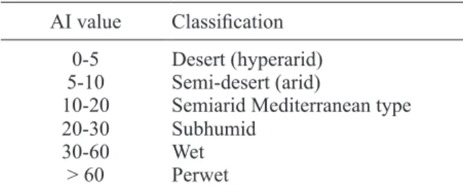
Where AI is the aridity index, which takes dimen-sionless values between 0 and > 60; MAR is the mean annual rain from historical records and the A2 scenario; MAT is the mean annual temperature from historical records and the A2 scenario; and 10 is a constant value derived from De Martonne’s model (Table I).
2.6 Origin and management of climate data
Data from 13 weather stations (WS) were used: 12 from the SMN and one from the Instituto Nacional de Investigaciones Forestales Agrícolas y Pecuarias (INIFAP, National Institute for Forestry, Agricultur-al and Livestock Research), located at the northern region of the municipality. All of them fell within a radius of approximately 65 km. Four WS correspond to the state of Coahuila (WS ID numbers: 5006, 5027, 5028 and 5029) and the other nine to the state of Durango. The metadata for the future scenarios are in this coverage as well (Fig. 3).
2.7 Indices related to edaphic properties and land use: CATEX and CAUSO
The estimated values of the indices CATEX and CAU-SO for the municipality of Gómez Palacio were created by manipulating the attribute tables of vector data sets containing the CATEX index. The indices were calcu-lated according to matching criteria between the type of soils used in Mexico by INEGI in the cartographic
Table I. De Martonne’s aridity index. AI value Classification
0-5 Desert (hyperarid) 5-10 Semi-desert (arid)
10-20 Semiarid Mediterranean type
20-30 Subhumid
30-60 Wet
> 60 Perwet
Source: http://www.miliarium.com/prontuario/Medio-Ambiente/Atmosfera/IndicesClima.htm#De_Martonne. DURANGO STATE COAHUILA STATE Mapimí Tlahualilo Gómez Palacio Leyend
WS, Id number Node scenarios GP, municipality Municipal limit 10085 10045 5028 5027 5006 10108 10049 10055
104 103.5 103
104 103.5 103
ºW ºN N 25 25. 52 6 25 25. 52 6 5029 Cuencame 10140 10009 Lerdo Nazas S. Bolivar NOR 10004 Weather stations (WS) selected to characterize the
climate of Gomez Palacio Id WS 5006 5027 5028 5029 10004 10009 10045 10055 10108 10140 10049 10085
Id WS= Identification key for WS; Coord= Coordinate; NOR = Not oficially registered in the WS-SMN.
Note:
WS and nodes distributed every 50 km for Future Scenarios 2010-2039.
NOR
WS Coordinates Height
Name x
103.400 25.533 1136 1116 1112 1276 1360 1135 1325 1330 1139 2230 1264 1096 1140 25.700 25.767 25.083 25.283 25.533 25.817 25.083 25.500 25.533 25.233 26.168 25.886 103.300 103.230 103.350 103.750 103.520 103.850 103.750 103.370 104.167 104.117 103.483 103.476
--- degrees --- m
y
Col. Torreón Jardín Presa Cuije Presa Guadalupe Presa La Flor Presa de Fernández Cd. Lerdo (SMN)
Cd. Lerdo (DGE) La Cadena Nazas Tlahualilo CNID-RASPA Mapimí (km 29) Pedriceñas
series I and II. Series I was elaborated based on the soils classification developed by FAO-UNESCO in 1968 and modified by CETENAL in 1970 (Krasil-nikov et al., 2013). Series II was based on the World Reference Base for Soils (FAO-ISRIC-ISSS, 1998). The soils of the municipality are almost entirely of calcareous origin, so we selected texture qualification and physical phase. The CAUSO index, associated with the distribution and abundance of vegetation, was estimated based on the identification of four vegetation groups, as well as the land dedicated to agricultural use and under irrigation (Table II).
2.8 Metadata for regionalized climate scenarios (2010-2039) to determine the LWE
To assess the climate changes, metadata were down-loaded from the SEMARNAT-INE website (http:// zimbra.ine.gob.mx/escenarios/) corresponding to MAT and MAR for three future scenarios: A2, A1B and B1 for the 2010-2039 period. In the original metadata, each one has a specific format; rain anomalies are in percent, and the temperature is in degrees Celsius (Table III).
The climatic future scenarios produced by Magaña and Caetano (2007), with anomalies for rain and temperature (shown in Table III), are the result of numerous experiments based on the 24 GCM proposed by the IPCC. In fact, this work is the origin of GHG emission lines (IPCC, 2007) whose characteristics are as follows:
Scenario A1: Assumes a very rapid global eco-nomic growth, up to doubling the world population by mid-century, and the rapid introduction of new and more efficient technologies. It is divided into three groups, which reflect three alternative directions for technological change: intensive fossil fuels (A1FI), non-fossil energy (A1T), and a balance between the various energy sources (A1B).
Scenario B1: Describes a convergent world with the same population as A1 but with a more rapid
evolution of economic structures toward a service and information economy.
Scenario A2: Describes a very heterogeneous world with strong population growth and both slow economic development and technological change.
2.9 Geostatistical analysis and assessing impact The impact analysis of future climate variability in rainfall and temperature began with the creation of a projected layer (shp), according to the locations (x, y) of the weather stations. The data were interpolated for each of the variables included in the study (zi), using an inverse distance-weighted (IDW) method in ArcMap 10 (ESRI), the same method used by Karaca (2012). The first product of this process was the creation of a raster layer adjusted to maximum and minimum extreme values. The second product was a change of the properties of the statistical and pixel raster image in tree classes for calculating the changes from historic or current data to the future scenarios. Next, we converted the classified raster image to a vector format, from which it was possible to determine the surface terms most impacted.
3. Results and discussion
The WS data set shown above (Table III) was calculated for each variable; for the mean annual rain-fall, percent anomalies were subtracted, and for the temperatures, the anomaly value was directly added. The percentage anomalies for both MAR and MAT were very similar among the three future scenarios described by Magaña and Caetano (2007), A2, A1B and B1. Therefore, this single study focused only on local impacts of the A2 scenario.
3.1 Analysis of the MAR impact
The values in Table IV, which compares the projected MAR to the historic (HMAR), are consistent with the maximum (287.5 mm) and minimum rainfalls
Table II. CATEX and CAUSO indexes.
CATEX TCPP C-INEGI, 2007 CAUSO Category and use
3.5 1 Coarse 0.70 C1, rainfed agriculture
1.75 2 Medium 0.20 C2, irrigated agriculture
1.85 3 Fine 0.15 C3, scrubland
0.87 SPB PPG 0.30 C4, grassland
Table III. HMAR and HMA
T and anomalies regionalized for Mexico for three future scenarios of the 2010-2039 period.
WS Id.
WS name
Coordinates
Elevation
m
MAR HMAR mm
Anomaly M AT HMA T Anomaly Long. W Lat. N A2 A1B B1 A2 A1B B1 Degrees % ºC 5006 Col. T orreón Jardín 103.4 25.533 1136 256.2 –2.55 –3.08 –2.79 22 0.86 0.926 0.838 5027 Presa Cuije 103.3 25.7 111 6 194 –3.32 –3.08 –2.79 21.9 0.86 0.926 0.838 5028 Presa Guadalupe 103.23 25.767 111 2 203.3 –3.32 –3.08 –2.79 21.5 0.86 0.926 0.838 5029
Presa La Flor
103.35 25.083 1276 280.3 –2.55 –2.87 –2.94 20.9 0.856 0.929 0.836 10004
Cañón de Fernández
103.75 25.283 1360 320.4 –3.98 –3.94 –3.69 22.1 0.867 0.935 0.835 10009
Cd. Lerdo (SMN)
103.52 25.533 1135 286.6 –2.98 –2.95 –2.24 21 0.851 0.926 0.823 10045
Mapimí (km 29)
103.85 25.817 1325 320.1 –2.98 –2.95 –2.24 19.3 0.851 0.926 0.823 10055 Pedriceñas 103.75 25.083 1330 403.6 –3.98 –3.94 –3.69 19.6 0.867 0.935 0.835 10108
Cd. Lerdo (DGE)
103.37 25.5 1139 270.1 –2.55 –2.87 –2.94 21 0.856 0.929 0.836 10140 La Cadena 104.167 25.533 2230 274.2 –3.76 –2.84 –2.73 21.2 0.865 0.973 0.834 10049 Nazas 104.1 17 25.233 1264 348.9 –2.81 –2.95 –2.61 20.3 0.883 0.958 0.85 10085 Tlahualilo 103.483 26.168 1096 266.4 –1.64 –2.12 –2.74 20.6 0.861 0.92 0.827 NOR CENID-RASP A 103.476 25.886 1127 209.6 –3.32 –3.07 –2.78 20.5 0.86 0.926 0.838 Aver . 1280 279.5 –3.06 –3.06 –2.84 20.9 0.861 0.933 0.835 Stdev 301 59.46 0.66 0.46 0.44 0.86 0.008 0.015 0.007 WS Id.: W eather station key; Aver .: Average; Stdev: Standard deviation; NOR: Not officially registered in the WS-SMN; HMAR: Historic
for mean annual rainfall; HMA
(202.9 mm) in the 13 WS included in the present study. For the future scenario A2 (MARScA2), which is
given by subtracting the average negative anomalies, the lower limit (196.4 mm) is more affected, with a likely decrease of 6.5 mm per year.
Compared to HMAR, in the MARScA2,the impact
of such anomalies on the spatial distribution of the gradient in annual rainfall from west to east (Fig. 4b) is to decrease MAR for both the lower and upper ranges, at 6.5 and 9 mm, respectively, which equals an average impact of 3.16% (Table IV).
To complement the analysis of the changes in MAR from HMAR to 2039 (the A2 scenario), an additional digital process was performed over the “raster” images that represent the distribution of the HMAR with the objective of comparing similar ranges. Data for each time period was reclassified into three categories, and the involved surfaces were calculated (Fig. 4c).
We then compared the historical number of pixels and the surface area in each category to the projected scenario. Pixels from each period were divided into three classes (a1, a2, and a3 for HMAR and b1, b2, and b3 for MARScA2). The lowest category included
lower values in MARScA2. From HMAR to A2, 52%
of the surface shifted from class 1 to 2, and between class a3 and b3, the surface lowered 17.73%. In sce-nario A2, the class with the lowest values for MAR (196.4-237.6) the surface area increased 8.20%, while the surface of the class with the highest values (259.7-278.2) decreased (17.73%), changing from 39 887 to 24 955 ha. It is also important to mention the following:
The average MAR decreased 11.2 mm, to move from 248.5 to 237.3 mm annually between historical values and the future (Fig. 4c).
In the above-mentioned class with the highest values (259.7-278.2), the affected area extends from
the eastern boundary with the municipality of Mat-amoros, Coahuila, to the north by Tlahualilo, to the western boundary near Arcinas and Pastor Rovaix, and to the north near Lucero and Banco Nacional (Fig. 4b).
There is a concentration of pixels in the lower range in scenario A2 (b3), which magnifies the im-pact. Although the mean difference between a3 and b3 is 8.9 mm, the impact is much greater because of the number of values concentrated towards the lower limit of that range (Fig. 4d).
Finally, it is important to note the anomalies affecting two WS: Cañon de Fernández (Id. 10004) and Pedriceña (Id. 10055). At these stations, runoff of surface water begins to feed the reservoirs (Francisco Zarco dam), and the agricultural irrigation of Gómez Palacio depends on this runoff. In absolute terms, the MAR could exceed the average for the three scenar-ios; i.e., the consequence of this declination index is approximately 4%.
3.2 Calculation and zoning of the GROPE
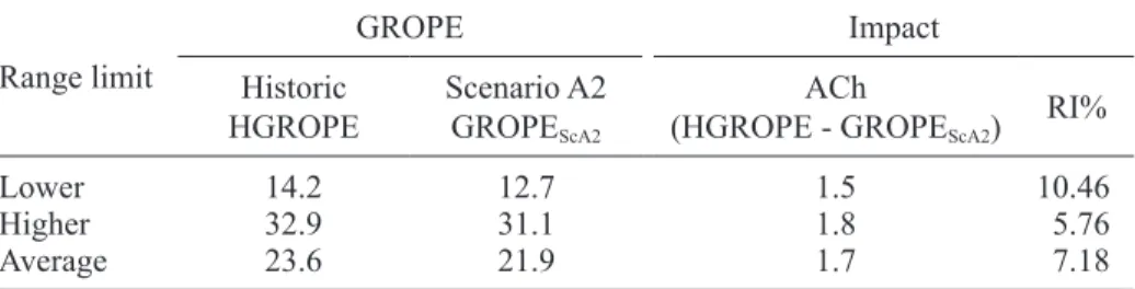
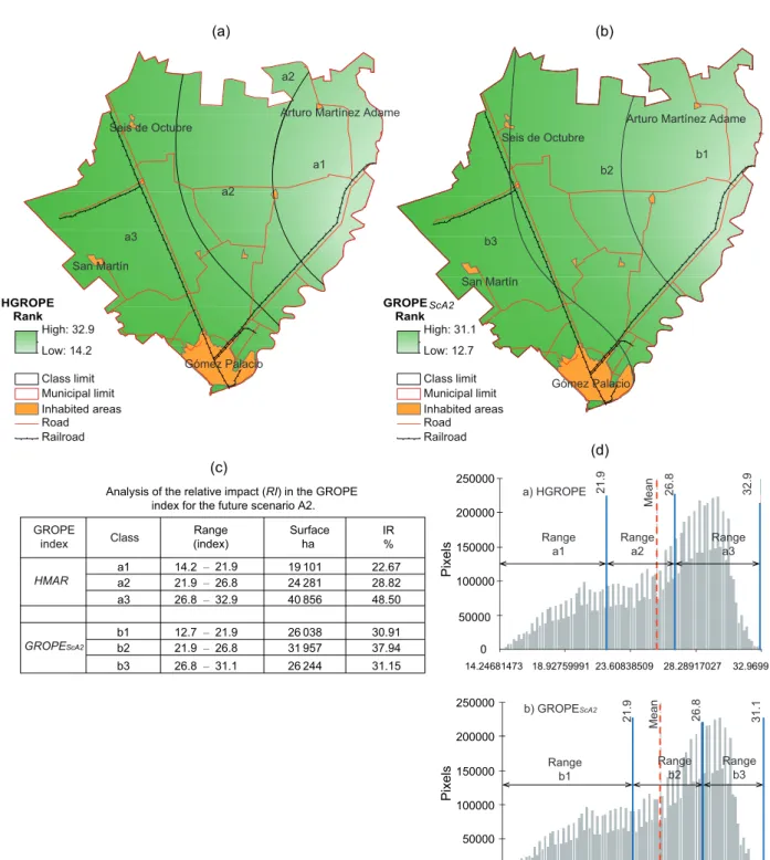
The GROPE is an index that was calculated based on Eq. (1), where the independent variable is the MAR. Therefore,it compares anomalies in average annual rainfall in historical and the future scenario A2. We
compared HGROPE to GROPEScA2. The HGROPE
index fell by an average of 7.18% in the future A2 scenario (GROPEScA2). In addition, the boundaries
of the ranges change between the historic values (14.2-32.9) and the GROPEScA2 (12.8-31.1), as shown
in Table V.
Based on the relationship that exists between the MAR and GROPE index, we would expect the MAR to be affected to the same extent, although it is not easy to determine the magnitude of the impacts of this signal in the limits of the range considered. To clarify
Table IV. The relative impact (RI) on MAR in the future scenario A2.
Range
MAR Impact
Historic
(HMAR) A2 (MARScenarioScA2)
ACh
(HMAR – MARScA2) RI
% mm
Lower 202.9 196.4 6.5 3.2
Upper 287.5 278.5 9 3.13
Average 245.2 237.4 7.75 3.16
Class Rangemm Surfaceha IR%
19601
HMAR 24750
39887
26505
MARScA2 32777
24955
Analysis of the relative impact (IR) on mean annual rainfall (MAR) for the future scenario A2
– – – – – –
a1 a2 a3
b1 b2 b3
23.27 29.38 47.35
31.46 38.91 29.62 202.9
237.6 259.7 259.7 287.1
196.4 237.6 237.6 259.7 259.7 278.2 237.6
287.1 202.9 Inhabited areas Municipal limit Road Railroad Class limit
Rank, mmHMAR
a3
a2
a1
a2
Arturo Martínez Adame
Seis de Octubre
San Martín
Gómez Palacio
b1 b2
b3
Seis de Octubre Arturo Martínez Adame
San Martín
278.5 196.4 Inhabited areas Municipal limit Road Railroad Class limit
Rank, mm MARScA2
(b) (a)
(c) (d)
Gómez Palacio
Rain, mm
Pixels
250000
200000
150000
100000
50000
0 200000
250000
150000
100000
50000
202.9968567 224.0277023 225.058548 266.0893936 287.120239
196.4049835 216.8509729 237.2969624 257.7429518 278.188941
0
Pixels
a) HAAR
Range a1
Range b1
Range a2
Range b2
Mean
Mean
Range b3 Range a3
b) A2 AAR
237.
6
237.
6
259.
7
259.
7
281.
7
281.
7
Mean annual rainfall,
MAR
Fig. 4. Spatial distribution of HMAR (a) and MARScA2 (b); impact analysis based on surface and relative impact
this in terms of the impact at the surface level (Fig. 5) that would be affected, the GROPE index images were also reclassified into three classes (Fig. 5c) and compared.
First,between classes a1 and b1, there is a project-ed increase of 6937 ha, equivalent to 8.23%, which would imply an extension of 2.7 km from east to west. This extension would occur from Esmeralda, where currently the HGROPE is located, to the west in the vicinity of Pastor Rovaix and Consuelo. Second, be-tween classes a2 and b2, there is a projected increase of 7676 ha, equivalent to 9.11%, which would imply an extension of approximately 5 km from east to west. This extension would occur from La Popular, which is currently HGROPE, to the west near to El Cairo, Estación Noé, La Plata and Bucareli. Third, there is a double impact in the shift between classes a3 and b3. The GROPE index would have a reduction of two units from the HGROPE (26.8-32.9) to the GROPEScA2 (26.8-31.1), and the index also has lower
maximum values in class b3 (Fig. 5d).
3.3 Calculation and zoning of the WAI
As in the previous cases, the WAI could be affected in the future A2 scenario (WAIScA2) because of the
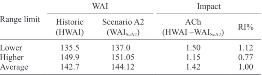
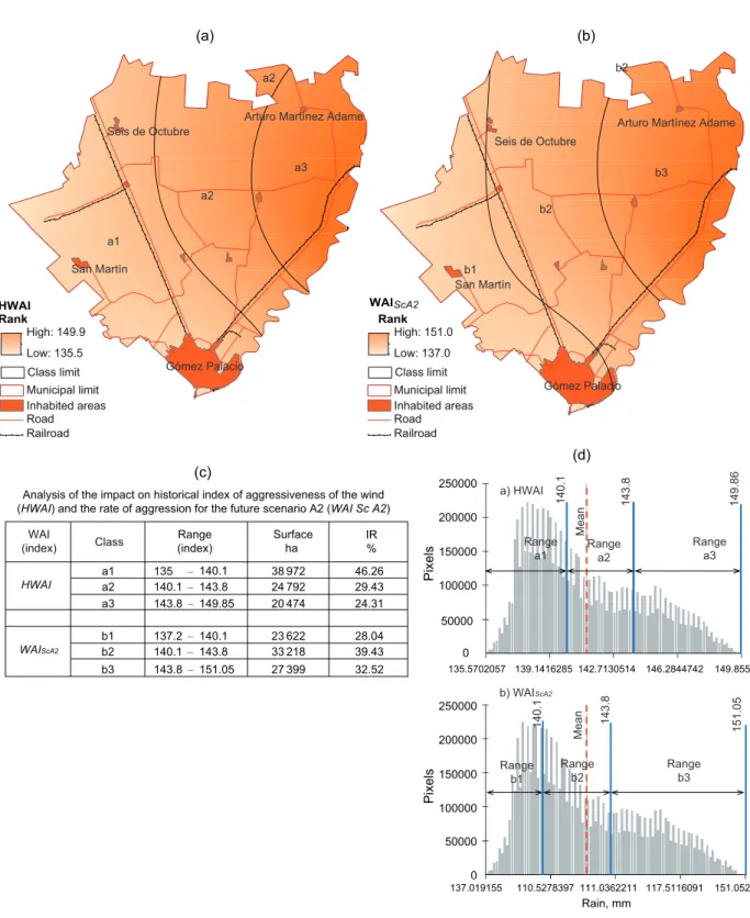
way the MAR is affected, although the relationship is more direct for GROPE as described in the meth-odology (Eq. 1). WAI could therefore be impacted in climate scenario A2 for the territory of Gómez Palacio by an average reduction of 1% and a change in the range of values from historical levels (135.5-149.9) to the A2 scenario (137-151.05), as shown in Table VI.
The spatial distribution of the WAI is presented in Figure 6. One salient change is the growth between classes a2 and b2, which is estimated to affect a total of 33 218 ha, derived from an increase of 10% between HWAI and WAIScA2 (Fig. 6c). This increase
includes the area known as Perímetro Lavín, where the following stations are located: El Cairo, Com-petencia, Noé, Dolores, Numancia and Britingham (Fig. 6b).
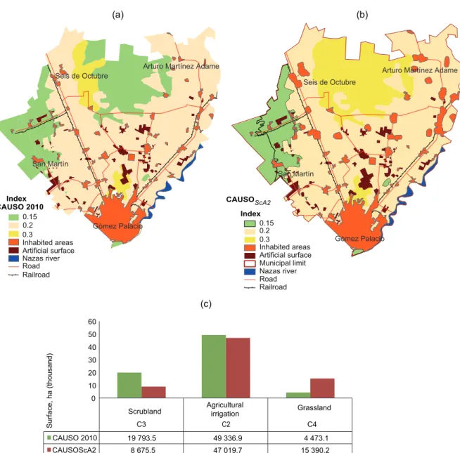
3.4 Calculation and zoning of the CAUSO index The CAUSO is an index defined by current land use (Table II), and the determination of the surfaces that will be occupied by urban nuclei on a horizon of approximately 30 years (2010-2039) was based on the programa de desarrollo urbano (PDU, program of urban development) of the municipality of Gómez Palacio (SEMARNAT, 2012). The distribution of the CAUSO index is shown in Figure 7, where future im-pacts can be assumed because of the drastic changes in categories C3 and C4. For the first category, there is a probable decrease in scrubland located in the western part of the municipality near Poanas, Dina-mita and San Martín. The extent would fall from the 19 793.5 ha (26.9%) currently estimated to 8675.5 ha (12.2%) by 2035. For the second category, there is an estimated increase in the vegetation associated with sandy deserts (Halophyte) in the north of the municipality, which would grow from 4473.1 ha (6.1%) to 15 390.1 ha (21.7%) (Fig. 7c).
3.5 Estimation and zoning of the LWE rate
The rate ofLWE not only represents the quantity of soil loss per year but is also a way to evaluate envi-ronmental loss. To determine the LWE rate, a digital process was conducted based on algebra maps using matrix operations and between digital layers (raster) using Eq. (4). The inputs described above in the context of the A2 scenario were used, as in CAUSO and WAI, with the exception of the edaphic index (CATEX). Edaphic characters such as the texture and the physical phase (stoniness factor) are changes not easily predictable in a short period of time.
Table V. Impact analysis in the GROPE index as a result in the MAR changes.
Range limit
GROPE Impact
Historic
HGROPE Scenario A2GROPEScA2
ACh
(HGROPE - GROPEScA2) RI%
Lower 14.2 12.7 1.5 10.46
Higher 32.9 31.1 1.8 5.76
Average 23.6 21.9 1.7 7.18
Class (index)Range Surfaceha IR%
19101
HMAR 24281
40856
26038
GROPEScA2 31957
26244 Analysis of the relative impact (RI) in the GROPE
index for the future scenario A2.
– – – – – –
a1 a2 a3
b1 b2 b3
22.67 28.82 48.50
30.91 37.94 31.15 14.2
21.9 26.8 26.8 32.9
12.7 21.9 21.9 26.8 26.8 31.1 21.9
Rain, mm 250000
200000
150000
100000
50000
0 50000
202.9968567 224.0277023 225.058548 266.0893936 287.120239
196.4049835 216.8509729 237.2969624 257.7429518 278.188941
0
Pixels
250000
200000
150000
100000
Pixels
a) HGROPE
Range a1
Range b1
Range a2
Range b2
Mean
Mean
Range b3 Range a3
b) GROPEScA2
21.9
21.9
26.8
26.8
32.9
31.1
GROPE index
a3
a2
a1 a2
Seis de Octubre
San Martín
b3
b2
b1 Seis de Octubre
Arturo Martínez Adame
San Martín
Gómez Palacio
GROPE ScA2
Rank
High: 31.1 Low: 12.7
Class limit Municipal limit Inhabited areas Road Railroad
HGROPE Rank
High: 32.9 Low: 14.2
Class limit Municipal limit Inhabited areas Road Railroad
(b) (a)
(c) (d)
Arturo Martínez Adame
Gómez Palacio
14.24681473 18.92759991 23.60838509 28.28917027 32.9699
12.75743484 17.33757305 21.91771126 26.49784946 31.0779
Fig. 5. Spatial distribution of HGROPE (a) and GROPEScA2 (b); impact analysis based on surface and relative
Table VI. Impact analysis of the WAI as a consequence of the GROPE changes on the municipality of Gómez Palacio.
Range limit
WAI Impact
Historic
(HWAI) Scenario A2(WAIScA2)
ACh
(HWAI –WAIScA2) RI%
Lower 135.5 137.0 1.50 1.12
Higher 149.9 151.05 1.15 0.77
Average 142.7 144.12 1.42 1.00
RI% = (ACh/HGROPE)*100.
The results indicate an average impact on the order of 63.06%, derived from a change in the range in the historical laminar wind erosion (HLWE) rate from 36-106 to 36-151.4 t ha–1 yr–1 in the future for
the A2 scenario (LWEScA2), as shown in Figure 8c.
A more detailed analysis of the impact associat-ed with the increasassociat-ed susceptibility of soils to wind erosion and by a lower availability of moisture because of the lower MARScA2 indicates that this
effect might be great and could influence nearly one third of the municipality (Fig. 8d). The spatial distribution of the three classes of erosion is shown in Figure 8b.
3.6 Analysis of the variables related to the aridity index
In addition to the calculation for LWE, as shown above, the aridity index provides a good complement to determine the magnitude of probable impacts for decreasing MAR and increasing MAT. AI has been examined in the three climate scenarios analyzed for the north and northeast of Mexico (Magaña and Caetano, 2007; Magaña et al., 2012).
3.7 Changes in mean annual temperature
According to the climate scenarios in the report of the IPCC (2007), the mean temperature in the northern hemisphere during the second half of the 20th cen-tury was likely higher than any other 50 year period in the last 500, and most likely the highest over the past 1300 years.
According to the IPCC report (2007), significant changes were observed in the data for physical (snow, ice and frozen ground; hydrology; and coast-al processes) and biologiccoast-al systems (land, marine and freshwater biological systems), and there was great variation in the air surface temperature during the period 1970-2004. The temperature changed on
the order of 1 to 2 ºC within 200 km to the north of the Tropic of Cancer (23.5º N). This increase will affect almost all of the municipality, but especially the northern area, where Seis de Octubre and Arturo Martínez Adame are located.
Temperature and rain are obviously fundamental variables in the analysis of the deterioration of natural resources. Both are processed for the historic data set and later were calculated since the anomalies. The re-sults in Table III suggest that the temperature change estimated by HMAT would be from 21 to 21.8 ºC in the future A2 scenario (MATScA2).
3.8 Changes in the aridity index
Given the relationship the De Martonne model (Eq. 5) establishes for MAR and MAT, as mentioned above, a decrease of rain will accompany an increase in temperature. In a future scenario there may be en-vironmental deterioration manifested by an increase in aridity and prolonged drought as reported previ-ously for North America and particularly for Mexico (Frederick and Gleick, 2001; UACH-CONAZA- SEDESOL-SAGARPA, 2004; IPCC, 2008).
According to the calculations made from anom-alies already described for the MAR and the MAT (Table III), the aridity index in the municipality of Gómez Palacio would change from the historic values (HAI) of 9.3 to 8.7 in the future scenario A2 (AIScA2).
It is estimated that the average impact on this index in the future could be –0.53 ± 0.2 (Table VII).
Class (index)Range Surfaceha IR%
38972
HWAI 24792
20474
23622
WAIScA2 33218
27399
– – – – – –
a1 a2 a3
b1 b2 b3
46.26 29.43 24.31
28.04 39.43 32.52 135
140.1 143.8 143.8 149.85
137.2 140.1 140.1 143.8 143.8 151.05
140.1
Rain, mm 250000
200000
150000
100000
50000
0 50000
202.9968567 224.0277023 225.058548 266.0893936 287.120239
196.4049835 216.8509729 237.2969624 257.7429518278.188941
0
Pixels
250000
200000
150000
100000
Pixels
a) HWAI
Range
a1 Rangea2
Range b2
Mean
Mean
Range b3
Range a3
b) WAIScA2
140.
1
140.
1
143.
8
143.
8
149.86
151.05
WAI (index)
WAIScA2
Rank
Class limit
Rank
High: 149.9 Low: 135.5
Municipal limit Inhabited areas Road Railroad
(b) (a)
(c) (d)
HWAI
Class limit High: 151.0 Low: 137.0
Municipal limit Inhabited areas Road Railroad a1
a2
a3 a2
Seis de Octubre
Gómez Palacio
Arturo Martínez Adame
San Martín
b2
b3
b1
b2
Seis de Octubre
Arturo Martínez Adame
San Martín
Gómez Palacio
Analysis of the impact on historical index of aggressiveness of the wind (HWAI) and the rate of aggression for the future scenario A2 (WAI Sc A2)
135.5702057 139.1416285 142.7130514 146.2844742 149.85589
137.019155 110.5278397 111.0362211 117.5116091 151.05299
Range b1
Fig. 6. The spatial distribution of HWAI (a) and WAIScA2 (b); analysis of relative impact (RI) based on affected surface
It is also important to mention that in addition to the reduction in the range of index values from his-torical levels (6.5-9.62) to the future scenario AIScA2
(6.11-9.17), the average of this index changed from 8.06 to 7.64. Additionally, there is greater aridity in the highest class, as seen in the density of pixels between the two cases (Fig. 9d).
3.9 Environmental quality analysis and probable impacts
Environmental quality is a term that relates to certain conditions of “comfort” for people and natural envi-ronments or biological systems. The critical elements
are the availability of fresh water, air quality and temperature (Karaca, 2012; Kuo-Jen et al., 2012). The water in the form of rain becomes important in regulating temperature and its relationship with extreme events, such as drought and dust storms, among others (Sun et al., 2003; Batjargal et al., 2006; Zhang et al., 2012).
Arid and semiarid regions will likely experience an increase in temperature and decrease in rain (Rive-ra et al., 2007; García-Páez and Cruz-Medina, 2009; Magaña et al., 2012), especially for latitudes similar to the Bolsón de Mapimí, the area where Gómez Palacio is located.
ScA2
Index Index
0.15
Inhabited areas Artificial surface Municipal limit Nazas river Road Railroad
n
CAUSO
(b)
(c) (a)
Seis de Octubre
Gómez Palacio
Arturo Martínez Adame
San Martín
Seis de Octubre
Arturo Martínez Adame
San Martín
Gómez Palacio 0.15
Road
CAUSO 2010
Inhabited areas Artificial surface Nazas river Railroad 0.3
0.2 0.2
0.3
Scrubland Agriculturalirrigation Grassland
C3 C2 C4
CAUSO 2010 19 793.5 CAUSOScA2 8 675.5
49 336.9 47 019.7
4 473.1 15 390.2 0
10 20 30 40 50 60
Surface, ha (thousand)
Figure 7. Spatial distribution of CAUSO current (a) and CAUSOScA2 (b); impact analysis based on surface and
Although this study used an average temperature increase of less than < 1 ºC and a rainfall decline of approximately 3%, the changes may be larger. For example, Magaña et al. (2012) remarked that for the north of Mexico in the future A2 scenario, the aver-age temperature towards the end of the 21st century could increase from 3.5 ºC (± 0.6), with extremes for the drier months (March, April and May) up to 7 ºC, while rainfall could decline by up to 5%.
This decrease in humidity, as shown in Figure 8, could not only negatively impact the rates of soil erosion, with probable losses in the future scenario A2 of up to 151.4 t ha–1 yr–1, but could also result
in changes in the systems of biological feedback (Breshears et al., 2003; Harper et al., 2010), a crisis
of freshwater availability and negative effects on the air quality due to a drastic increase in suspend-ed particles. This change is potentially harmful to people´s health (Razo et al., 2004; Rashki et al., 2011) and could affect the albedo at the level of the surface of the Earth and the atmosphere (Batjargal et al., 2006; Hak-Sung et al., 2011). Figure 10 shows an aerial view of Gómez Palacio municipality and an example of qualitative laminar wind erosion.
The rate of laminar wind erosion was 151.4 t ha–1
yr–1, equivalent to the removal and transport of a soil
layer between 12.6 and 13.7 mm thick. If the soil is medium textured over the entire area of study, this amount is between 1100 and 1200 kg m–3, which
implies a potential loss of approximately 0.4 m in
ScA2
(b)
(c) (d)
(a)
Seis de Octubre
Arturo Martínez Adame
San Martín
Gómez Palacio
LWE Class
Low Moderate High
Inhabited areas (2035) Artificial surface Municipal limit Nazas river Road Railrad
HLWE Class
Low Moderate High
Inhabited areas (2010) Artificial surface Municipal limit Nazas river Road Railrad
Seis de Octubre
Gómez Palacio
Arturo Martínez Adame
San Martín
Analysis impact of the LWE in the future A2 scenario Rank From to --- Impacts --- limit LWEScA2 ACh RI
--- t ha yr --- % Lower 36 36 0 0 Upper 106 151.4 45.4 126.11
Average 71 93.7 22.7 63.06
HLWE
-1 -1
Changes between class erosion to HLWE and LWEScA2
Period Rank Surface RI Class (t ha-1 yr-1) ha %
Low 23 435 28.7 Moderate 55 130 67.6
High 3 023 3.7
Low 7 303 10.4
Moderate 45 950 65.1 High 17 296 24.5
HLWE
LWEScA2
36 - 41 41 - 55 55 - 106
36 - 41 41 - 55 55 - 151.4
Fig. 8. Spatial distribution of HLWE (a) and LWEScA2 (b); impact analysis based on surface and relative importance
30 years. For this type of soil, these values exceed the rates of soil loss tolerance (5-12 t ha–1 yr–1)
pro-posed by the United States Department of Agriculture (USDA) (Montgomery, 2007).
An example of changes in the biological feedback is that the removal of the soil directly affects the role of nitrogen (N). N determines plant productivity, and in arid environments, the soil frequently presents large accumulations of calcium carbonate that push the soil pH to a range of 7 to 8. At this pH, phosphorus (P) is in complex forms and not available (Munson et al., 2011; Schlesinger et al., 2011), a set of conditions that matches the selection criteria of the parameters for the CATEX index that was described in the methodolo-gy. In response to a deficiency of N and P, Larrea tridentata shows the highest levels of efficient use of nutrients that have been found in woody plants.
4. Conclusions
The models for the LWE and the AI suggest that in the immediate future (2010-2039) the climatic conditions of the area of study and its surroundings will deteriorate and could lead to a steady decline of environmental quality and health. There are two
important implications of this study. First, the mod-els can serve to warn people of the risks to human and natural environments from extreme conditions such as droughts and dust storms. Secondly, it is possible to identify local changes in use of the soil and deforestation.
Finally, it is important to mention that the mag-nitude and distribution of the impact on the territory are relevant to planning the management of natural resources. This research should be taken into account in decision-making about preventing impacts on natural resources now and in the future.
Acknowledgements
This article is part of the results of the research carried out within the framework of the Programa Estatal de Acciones ante el Cambio Climático (State Program of Action on Climate Change) Durango (PEACC-DGO) and Aguascalientes (PEACC-AGS) during a post-doctoral stay conducted between 2011 and 2012. Thanks to Joaquín Pinto Espinoza and Adriana Martínez Prado, both responsible for the PEACC-DGO, and Elsa Marcela Ramírez López, head of PEACC-AGS.
Table VII. Estimation of changes in the AI from the historic (HAI) to future A2 scenario (AIScA2) in Gómez
Palacio.
WS Id. NameWS-SMN
Coordinates Aridity Index
Long. Lat. HAI AIScA2 ACh
Degrees Index
5006 Col. Torreón Jardín 103.400 25.533 8.0 7.6 0.41
5027 Presa Cuije 103.300 25.700 6.1 5.7 0.36
5028 Presa Guadalupe 103.230 25.767 6.5 6.1 0.38
5029 Presa La Flor 103.350 25.083 9.1 8.6 0.47
10004 Cañón de Fernández 103.750 25.283 10.0 9.3 0.65
10009 Cd. Lerdo (SMN) 103.520 25.533 9.2 8.7 0.52
10045 Mapimí (km 29) 103.850 25.817 10.9 10.3 0.62
10055 Pedriceña 103.750 25.083 13.6 12.7 0.91
10108 Cd. Lerdo (DGE) 103.370 25.500 8.7 8.3 0.45
10140 La Cadena 104.167 25.533 8.8 8.2 0.56
10049 Nazas 104.117 25.233 11.5 10.9 0.64
10085 Tlahualilo 103.483 26.168 8.7 8.3 0.38
NOR CENID-RASPA 103.476 25.886 6.9 6.5 0.4
Aver. 9.3 8.7 0.53
Stddev 2.1 2.0 0.20
ACh: Absolute change on aridity index (HAI – AIScA2); the value of the historic temperature (bold) for the
Class Rankindex Surfaceha RI%
8209.7
HAI 25066.9
50984.5
21288.9
AIScA2 23998.5
38981.6
– – – – – –
High Moderate
Low
High Moderate
Low
9.74 29.75 60.51
25.26 28.48 46.26 6.5
7.7 8.5 8.5 9.62
6.11 7.7 7.7 8.5 8.5 9.62
7.7
202.9968567 224.0277023 225.058548 266.0893936 287.12023
196.4049835 216.8509729 237.2969624 257.7429518 278.18894
Pixels
Pixels
a) HAI
Range High
Range Moderate
Range Low
Range High
Range Moderate
Range Low
Mean
Mean
b) AIScA2
7.
7
7.
7
8.
5
8.
5
9.62
9.17
Period
ScA2
Clase
(b) (a)
(c) (d)
6.555311203 7.323812962 8.09231472 8.860816479 9.62931
6.118026257 6.880219316 7.642412376 8.4046054636 9.16679
AI
Seis de Octubre
Arturo Martínez Adame
San Martín
Gómez Palacio Low
Moderate High
Inhabited areas (2035) Artificial surface Municipal limit Road railroad
ClaseHAI
Low Moderate High
Inhabited areas (2010) Artificial surface Municipal limit Road railroad
Seis de Octubre
San Martín
Arturo Martínez Adame
Gómez Palacio
Analysis of the relative impact (RI) in the aridity index (AI) to the future scenario A2 (IAScA2).
150
100
50
0
150
100
50
0
Fig. 9. Spatial distribution of HAI (a) and AIScA2 (b); impact analysis based on surface and relative importance
Fig, 10. Current aerial view at different scales of the superficial area of Gómez Palacio and a close-up to the high critical zone of laminar wind erosion.
Scrubland & agricultural irrigation. Scale 500 m
Scrubland Scale 500 m
Municipal limit Scale 22.9 km
References
Batjargal Z., J. Dulam and Y. S. Chung, 2006. Dust storms are an indication of an unhealthy environment in East Asia. Environ. Monit. Assess. 114, 447-460, doi:10.1007/s10661-006-5032-3.
Breshears D. D., J. J. Whicker, M. P. Johansen and J. E. Pinder, 2003. Wind and water erosion and transport in semi-arid shrub land, grassland and forest ecosystems: Quantifying dominance of horizontal wind-driven transport. Earth Surf. Proc. Land. 28, 1189-1209, doi:10.1002/esp.1034.
FAO-ISRIC-ISSS, 1998. World reference base for soil resources. World Soil Resources Reports 84. Food and Agriculture Organization of the United Nations, Rome. Available at: http://www.fao.org/docrep/W8594E/ W8594E00.htm.
Frederick K. D. and P. H. Gleick, 2001. Potential impacts on US water resources. In: Climate change, science strategy and solutions (E. Claussen, V. Arroyo Cochran and D. P. Davis, Eds.). The Pow Center on Global Climate Change. Brill, Boston, pp. 63-82.
García E., 2003. Distribución de la precipitación en la República Mexicana. Investigaciones Geográficas
50, 67-76.
García-Páez F. and I. R. Cruz-Medina, 2009. Variabilidad de la precipitación pluvial en la región Pacífico norte de México. Agrociencia 43, 1-9.
Hak-Sung K., C. Yong-Seung and L. Sun-Gu, 2011. Char-acteristics of aerosol types during large-scale transport of air pollution over the Yellow Sea region and at Cheongwon, Korea, in 2008. Environ. Monit. Assess.
184, 1973-1984, doi:10.1007/s10661-011-2092-9. Harper R. J., R. J. Gilkes, M. J. Hill and D. J. Carter,
2010. Wind erosion and soil carbon dynamics in south-western Australia. Aeolian Research1, 129-141, doi:10.1016/j.aeolia.2009.10.003.
INE, 1998. Ordenamiento ecológico del territorio. Me-moria técnica y metodológica. Instituto Nacional de Ecología, Secretaría de Desarrollo Social, México, 66 pp.
to the Fourth Assessment Report of the Intergovern-mental Panel on Climate Change (M. L. Parry, O. F. Canziani, J. P. Palutikof, P. J. van der Linden and C. E. Hanson, Eds.). Cambridge University Press, Cam-bridge, 976 pp.
IPCC, 2007. Cambio climático 2007: Informe de síntesis. Contribución de los grupos de trabajo I, II y III al Cuarto Informe de Evaluación del Grupo Interguber-namental de Expertos sobre el Cambio Climático (R. K. Pachauri and A. Reisinger, Eds.). IPCC, Geneve, 104 pp.
Karaca F., 2012. Determination of air quality zones in Turkey. JAPCA J. Air Waste Ma. 62, 408-419, doi:10.1080/10473289.2012.655883.
Krasilnikov P., M. C. Gutiérrez-Castorena, R. J. Ahrens, C. O. Cruz-Gaistardo, S. Sedov and E. Solleiro-Rebolle-do, 2013. The soils of Mexico. World Soils Book Series. Springer, 175 pp., doi:10.1007/978-94-007-5660-1_2. Kuo-Jen L., P. Amar, E. Tagaris and A. G. Russell, 2012.
Development of risk-based air quality management strategies under impacts of climate change. JAPCA J. Air Waste Ma. 62, 557-565, doi:10.1080/10962247.2 012.662928.
Magaña V. O., J. L. Vázquez, J. L. Pérez and J. B. Pérez, 2003. Impact of El Niño on precipitation in Mexico.
Geofí. Int. 42, 313-330.
Magaña V. O. and E. Caetano, 2007. Pronóstico climático estacional regionalizado para la República Mexicana como elemento para la reducción de riesgo, para la identificación de opciones de adaptación al cambio climático y para la alimentación del sistema: cambio climático por estado y por sector (informe final). Direc-ción General de InvestigaDirec-ción sobre Cambio Climático, SEMARNAT-INE. 41 pp.
Magaña V. O., 2010. Guía para generar y aplicar esce-narios probabilísticos regionales de cambio climáti-co en la toma de decisiones. Centro de Ciencias de la Atmósfera, Universidad Nacional Autónoma de México, 80 pp.
Magaña V. O., D. Zermeño and C. Neri, 2012. Climate change scenarios and potential impacts on water avail-ability in northern Mexico. Clim. Res. 51, 171-184, doi:10.3354/CR01080.
Mercado-Mancera G., E. Troyo-Diéguez, A. Aguirre-Gó-mez, B. Murillo-Amador, L. F. Beltrán-Morales and J. L. García-Hernández, 2010. Calibración y aplicación del índice de aridez de De Martonne para el análisis del déficit hídrico como estimador de la aridez y desertifi-cación en zonas áridas. Universidad y Ciencia26, 51-64.
Monterroso A. I., A. C. Conde, D. Rosales, J. D. Gómez and C. Gay, 2011. Assessing current and potential rain-fed maize suitability under climate change scenarios in Mexico. Atmósfera 24, 53-67.
Montgomery D. R., 2007. Soil erosion and agricultural sus-tainability. P. Natl. Acad. Sci. USA 104, 13268-13272. Munson S. M., J. Belnapa and G. S. Okinb, 2011. Re-sponses of wind erosion to climate-induced vegetation changes on the Colorado Plateau. P. Natl. Acad. Sci. USA 108, 3854-3859.
PNUD, 2005. Marco de políticas de adaptación al cam-bio climático: desarrollo de estrategias, políticas y medidas (B. Lim and E. Spanger-Siegfried, Eds.). Programa de las Naciones Unidas para el Desarrollo, New York, 274 pp.
Rashki A., C. J. Rautenbach, P. G. Eriksson, D. G. Kas-kaoutis and P. Gupta, 2011. Temporal changes of par-ticulate concentration in the ambient air over the city of Zahedan, Iran. Air Quality, Atmosphere & Health, doi:10.1007/s11869-011-0152-5.
Razo I., L. Carrizales, J. Castro, F. Díaz-Barriga and M. Monroy, 2004. Arsenic and heavy metal pollution of soil, water and sediments in a semi-arid climate mining area in Mexico. Water Air Soil Poll. 152, 129-152, doi:10.1023/B:WATE.0000015350.14520.c1. Rivera del Río R., G. Crespo Pichardo, R. Arteaga Ramírez
and A. Quevedo Nolasco, 2007. Comportamiento es-pacio temporal de la sequía en el estado de Durango, México. Terra Latinoamericana 25, 383-392. Rose C. W., 2005. Erosion by water, modeling. In:
Ency-clopaedia of Soil Science (R. Lal, Ed.). Marcel Decker, New York, pp. 468-472.
Schlesinger W. H., J. J. Cole, A. C. Finzi and E. A. Hol-land, 2011. Introduction to coupled biogeochemical cycles. Front. Ecol. Environ. 9, 5-8.
SEMARNAT, 2012. Estudio técnico para el ordenamiento ecológico y territorial del municipio de Gómez Pala-cio, Durango. Resumen ejecutivo. Secretaría de Medio Ambiente y Recursos Naturales, Secretaría de Recur-sos Naturales y Medio Ambiente de Durango, México, 265 pp. Available at: http://www.gomezpalacio.gob. mx/2010-2013/images/stories/ecologia/consulta/Re-sumen_Ejecutivo_Gomez_palacio.pdf [last accessed on March 5, 2013].
semarnat.gob.mx/informacionambiental/documents/ sniarn/pdf/Cuarta_Comunicacion_Nacional.pdf. SEMARNAT-INE, 2011. Sistema de información de
esce-narios de cambio climático regionalizados (SIECCRe). Metadatos y mapas para SIG. Available at: http:// zimbra.ine.gob.mx/escenarios/ [last accessed on Sep-tember 24, 2011].
Sun L., X. Zhou, J. Lu, Y-P, Kim and Y-Seung Chung. 2003, Climatology, trend analysis and prediction of sandstorms and their associated dust fall in China.
Water Air Soil Poll. 3. 41-50.
UACH-CONAZA, 2004. Escenarios climatológicos de la República Mexicana ante el cambio climático.
Universidad Autónoma Chapingo, Comisión Nacional de Zonas Áridas, México, 169 pp.
Van Roosmalen L., T. O. Sonnenborg, K. H. Jensen and J. H. Christensen, 2011. Comparison of hydrological simulations of climate change using perturbation of observations and distribution-based scaling. Vadose Zone J. 10,136-150, doi:10.2136/vzj2010.0112. Yu B., 2003. A unified framework for water erosion and
deposition equations. Soil. Sci. Soc. Am. J. 67, 251-257. Zhang Q., J. Li, V. P. Singh, C. Y. Xu and Y. Bai, 2012.
Changing structure of the precipitation process during 1960-2005 in Xinjiang, China. Theor. Appl. Climatol.