Fast computation of electromagnetic near-fields with the multilevel fast multipole method combining near-field and far-field translations

(1)

www.adv-radio-sci.net/4/111/2006/ © Author(s) 2006. This work is licensed under a Creative Commons License.

Radio Science

Fast computation of electromagnetic near-fields with the multilevel

fast multipole method combining near-field and far-field translations

A. Tzoulis1and T. F. Eibert2

1_{FGAN-Research Institute for High-Frequency Physics and Radar Techniques (FHR), Wachtberg-Werthhoven, Germany} 2_{Institute of Radio Frequency Technology, University of Stuttgart, Germany}

Abstract. In Electromagnetic Compatibility (EMC) prob-lems, computation of electromagnetic near-fields in the vicinity of complex radiation and scattering systems is of-ten required. Numerical solution of such problems is achieved using Boundary Integral (BI) based approaches, where the involved Integral Equations (IE’s) are solved with the Method of Moments (MoM). The MoM solution process is speeded up by fast IE solvers such as the Multilevel Fast Multipole Method (MLFMM). In the end the desired am-plitudes of the expansion of the equivalent current densities on the discrete elements all over the Huygens’ surfaces are known. Computation of the electromagnetic fields produced by the equivalent currents at observation points being in the near-field regions requires integration of the current densi-ties over the Huygens’ surfaces. Numerical evaluation of the near-field integrals using conventional integration rules can become extremely time consuming for large objects and large number of observation points. In this contribution, ac-celeration of the near-field integration of the equivalent cur-rent densities is provided using a postprocessing MLFMM, where near-field and far-field translations are combined in order to achieve optimum performance. The proposed ap-proach was applied in the postprocessing stage of a power-ful Finite Element Boundary Element (FEBI) method, result-ing in significant decrease of the postprocessresult-ing computation time. The formulation of the proposed acceleration is pre-sented and numerical results are shown.

1 Introduction

Complex radiation and scattering problems are solved these days routinely using Boundary Integral (BI) based methods, where the Integral Equation’s (IE’s) are solved by the Method of Moments (MoM) (Rao et al., 1982) using fast integral Correspondence to: A. Tzoulis ([email protected])

equation solvers like the Multilevel Fast Multipole Method (MLFMM) (Chew et al., 2001; Eibert, 2005). The MoM so-lution provides the desired amplitudes of the expansion of the equivalent current densities on the discrete elements all over the Huygens’ surfaces.

In order to compute the electromagnetic fields produced by the equivalent currents on observation points in the near-field region of the involved objects, integration of the current den-sities over the entire Huygens’ surfaces must be performed in the postprocessing stage. Such computations are needed in Electromagnetic Compatibility (EMC) problems like in-vestigations within cars or for safety assessment in the vicin-ity of mobile communications base station antennas. The complexity of evaluating near-field integrals in the postpro-cessing stage using conventional numerical integration rules isO(N M), whereN is the number of equivalent current el-ements and M the number of observation points. It is ob-vious that postprocessing computations become extremely time-consuming in case of large objects and large number of observation points.

(2)

ap-E

inc

_{, H}

inc

• • • • • •

closed surface

A

observation points

′ −

r r

( )

A ′ J r

( )

A ′ M r

• • • • • •

BI-MLFMM domain

near-field MLFMM translation domain far-field MLFMM translation domain

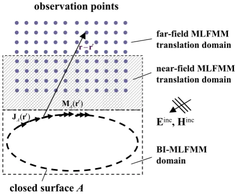
Fig. 1. Configuration for postprocessing computations of BI based

methods.

plied in the postprocessing stage of a powerful Finite Ele-ment Boundary EleEle-ment (FEBI) method (Jin, 1993; Volakis et al., 1998), resulting in significant decrease of the postpro-cessing computation time.

In the following, the formulation of the MLFMM ap-proach for the postprocessing stage is presented and numeri-cal results are shown.

2 Formulation

Consider the configuration of Fig. 1, where electricJA(r0) and magneticMA(r0)current densities are given all over the closed Huygens’ surfaceAand are known from the solution of any BI based method.

The electric and magnetic fields at an observation point

r produced by the surface currents are given by the integral expressions

E(r)=

ZZ

A

₋

GE_J(r,r0)·JA(r0)+

−

GE_M(r,r0)

·MA(r0)

da0+Einc(r) (1) and

H(r)=

ZZ

A

₋

GH_J(r,r0)·JA(r0)+

−

GH_M(r,r0)

·MA(r0)

da0+Hinc(r), (2)

respectively, where

−

GE/H_J (r,r0) and

−

GE/H_M (r,r0) are the Green’s functions of the electric or magnetic field due to elec-tric and magnetic surface currents, respectively. The equiv-alent currents onAare assumed to be available in a known

expansion using RWG basis functions on triangular surface elements according to

JA(r0)=

X

n

Jnβn(rn),

M_A(r0)= −X

n

Mnβn(rn). (3) The evaluation of the field contributions in Eqs. (1) and (2) is accelerated using MLFMM. According to this, the BI-MLFMM domain is extended towards the observation points and in addition to non-empty source groups containing cur-rents also non-empty receiving groups containing observa-tion points are collected on each level. The field contri-butions from source groups to non well-separated receiving groups are evaluated conventionally by numerical integration rules. All other field contributions at an observation point

r=rmare computed using the fast multipole representations

E(rm)= −j

ωµ

4π

Z

e−jk·rmm0_T

L(kˆ· ˆrm0_n0) −

I− ˆkkˆ

·X

n

Jn

∼

βn(k) dˆ kˆ2

−j k

4π

Z

ˆ

k×e−jk·rmm0_T

L(kˆ· ˆrm0_n0)

X

n

Mn

∼

βn(k) dˆ kˆ2+Einc(rm) (4) and

H(rm)= −j

k

4π

Z

ˆ

k×e−jk·rmm0_T

L(kˆ· ˆrm0_n0)

X

n

Jn

∼

βn(k) dˆ kˆ2

+jωε

4π

Z

e−jk·rmm0_T

L(kˆ· ˆrm0_n0) −

I− ˆkkˆ

·X

n

Mn

∼

βn(k) dˆ kˆ2+Hinc(rm), (5) where

∼

βn(k)ˆ = Z Z

A

βn(rn)ej k·rnn0dan (6)

is the kˆ-space representation of the source basis functions withk=kkˆ.TL(kˆ· ˆrm0_n0)is the conventional FMM diagonal

(3)

2 (1.7 )D

r

π

λ

≥

0 1 2 3 4 5 6

0 50 100 150 200 250

Fa

r-fie

ld c

ondition r

(m)

D (m)

λ=1 m

Fig. 2. Far-field condition with increasing group dimensions.

Extending the near-field translation domain to all obser-vation points can be extremely memory-consuming. There-fore, near-field MLFMM translations are applied only to nearby observation points and far-away observation points are preferably treated by far-field MLFMM translations, where the translation operator is approximated by a far-field representation only for the ray direction from the source group to the observation point. Thereby, it is assumed that the observation point lies in the far-field of the individual source group. The field contributions for an observation pointr=rmwithin the far-field MLFMM translation domain are given by

E(rm)= −j

ωµ

4πT

F F L (krmn0)

−

I− ˆk0kˆ0

·X

n

Jn

∼

βn(kˆ0)

−j k

4π

ˆ

k0×TLF F(krmn0) X

n

Mn

∼

βn(kˆ0)

+Einc(rm) (7)

and

H(rm)= −j

k

4π

ˆ

k0×TLF F(krmn0) X

n

Jn

∼

βn(kˆ0)

+jωε

4πT

F F L (krmn0)

−

I− ˆk0kˆ0

·X

n

Mn

∼

βn(kˆ0)

+Hinc(rm), (8)

whereT_LF F(krmn0)is the far-field MLFMM translation

oper-ator in the ray directionkˆ0= ˆrmn0 (Chew et al., 2002).

Im-proved far-field representation is obtained using the gravity center of the currents within the source groups as reference point for the radiated fields of the groups. The necessary ray directionkˆ0, which connects the gravity center of the currents within the source group with the observation point, is com-puted from the neighboring sampling points of the numerical integration in thekˆ-space by interpolation.

x y z

FEBI-MLFMM

13509 electric BI unknowns 10827 magnetic BI unknowns 118503 FE unknowns

3 λλλλ0

εεεε_r=2.5

f = 10 GHz

Fig. 3. Real part of surface current density on dielectric rod antenna.

The condition used to perform far-field translations is

rf ar≥

π(1.7DL)2

λ (9)

and is derived from the criterion for far-field translations according to the Fast Far-Field Approximation (FAFFA) in (Chew et al., 2002). DL is the group dimension on level

L and λ is the wavelength. The condition increases with the square of group dimensions, as shown in Fig. 2, which means that enforcing satisfaction of this condition for the whole scatterer or antenna would be very inefficient. It is rather assumed that far-field condition is satisfied by the in-dividual source groups on the various levels. For each obser-vation point, far-field translations are performed on the coars-est levelL, on which condition (9) is still satisfied. This level is found for each observation point in the initialization step in a worst-case sense using its shortest distance to the BI-MLFMM domain. Improved accuracy is provided by choos-ing a more strchoos-ingent far-field condition.

The proposed acceleration of near-field computations was applied at the postprocessing stage of a powerful FEBI method. In the next section numerical results showing the savings in computation time will be presented.

3 Numerical examples

(4)

x (m)

|

Ε

|(

d

B

)

0 0.1 0.2 0.3 0.4 0.5 0.6 0.7

-18

-16

-14

-12

-10

-8 -6 -4 -2 0

Numerical Integration 236.4 sec P-MLFMM

13.6 sec

Fig. 4. Electric field along the axis of dielectric rod antenna.

x (m)

y(

m

)

160

140

120

100

80

60

40

20

z=0.0 m |E| (V/m)

Fig. 5. Instantaneous electric field fort=0 s on the xy-plane.

conventional near-field integration. It can be seen that re-sults show excellent agreement and the P-MLFMM compu-tations need much less computation time. Further, the instan-taneous electric field fort=0 s can be seen in Fig. 5 on the xy-plane, cutting through the antenna in the middle along its axis. These computations were performed on 100701 obser-vation points with the P-MLFMM approach in about 7 min on an AMD Athlon 2800+ PC combining near-field and far-field translations. The wave radiated by the antenna mainly at the transition region between metallic mounting and electric material with very low radiation in the backward di-rection can be clearly seen.

Next example is the open metallic cuboid shown in Fig. 6. The length of the structure is 30λand the square cross sec-tion has an inner edge length of 10λ. The object is placed symmetrically to the xy-plane. In the same figure the mag-nitude of the surface current density on the metallic cuboid

x z

y

Einc

12 λλλλ

12 λλλλ λλλλ

30 λλλλ

|E0| = 1 V/m f = 3 GHz

897051 BI currents

Fig. 6. Magnitude of surface current density on open metallic 30λ cuboid.

y (m)

|

Εto

t

|(

V

/m

)

-2 -1.5 -1 -0.5 0 0.5 1 1.5 2

0 0.5

1 1.5

Numerical Integration 8.5 h P-MLFMM 0.5 h

Fig. 7. Total electric field along the y-axis for open metallic cuboid.

can be seen, which is the BI solution of 897051 surface cur-rents for vertically polarized plane wave excitation travel-ing towards the opentravel-ing of the cuboid. In the postprocess-ing stage, the electric field was observed along the y-axis on 10001 observation points by performing the computations with the fast postprocessing approach and with conventional near-field integration. The results are shown in Fig. 7, where excellent agreement and saving of large amount of computa-tion time can be seen. Further, the electric field was observed on a 2×4 m2window in the xy-plane with 1 mill. observa-tion points. The computaobserva-tions were performed with the P-MLFMM approach in about 8 h combining near-field and far-field translations. The estimated computation time with con-ventional numerical integration would be about 850 h, which is unacceptably high. The results are shown in Fig. 8, where the expected distribution of the electric field inside, outside and within the metallic walls of the cuboid can be seen.

(5)

x (m)

3.5

3.0

2.5

1.5

1.0

0.5

0.5 1.0 1.5 2.0

0.0 -0.5 -1.0 -1.5 -2.0 0.0 0.2 0.4 0.6 0.8 1.0

-0.2

-0.4

-0.6

-0.8

-1.0

y(

m

)

z=0.0 m |Etot| (V/m)

Fig. 8. Total electric field through the open metallic cuboid.

x

z

y

E

inc

BI-MLFMM

~ 6 Mio. BI unknowns

89 h, 17 GB RAM on Opteron 2.2 GHz CPU |E₀| = 1 V/m 30°°°°

f = 3.2 GHz

~ 17.5 m

Fig. 9. Full-scale Mig-29 model forf=3.2 GHz.

in Fig. 9. The model is about 17.5 m long and was excited by a vertically polarized plane wave traveling 150◦from the x-axis towards the nose of the aircraft. The BI solution of this problem was performed on an AMD Opteron 2.2 GHz CPU using about 6 mill. unknowns. In the postprocess-ing stage the near-field was observed through the aircraft on a plane parallel to the xy-plane on about 2.2 mill. ob-servation points. These computations were performed with the P-MLFMM approach in about 3 h, combining near-field and far-field translations. The magnitude of the total electric near-field through the Mig-29 is shown in Fig. 10, where the expected distribution of the electric field can be seen.

P-MLFMM on 2.2 Mio observation points 3 h, 8 GB RAM on Opteron 2.2 GHz CPU

x (m)

y(

m

)

10 0

15

0 5

1 2 3 4 5

-1

-4 -2

-3

-5

2.5

2.0

1.0 z=1.9 m |Etot| (V/m)

1.5

0.5

Fig. 10. Total electric field through Mig-29.

4 Conclusions

In this contribution, the multilevel fast multipole method was used to accelerate near-field computations in the postpro-cessing stage of boundary integral based methods for nu-merical solution of electromagnetic radiation and scattering problems, where optimum performance is achieved combin-ing near-field and far-field translations. The proposed P-MLFMM was applied in the postprocessing stage of a pow-erful FEBI method and numerical results were shown, where saving of large amount of computation time in the postpro-cessing stage could be clearly seen.

References

Chew, W. C., Jin, J.-M., and Michielssen, E.: Fast and efficient algorithms in computational electromagnetics, Boston: Artech House, 2001.

Chew, W. C., Cui, T. J., and Song, J. M.: A FAFFA-MLFMA al-gorithm for electromagnetic scattering, IEEE Trans. Antennas Propagat., 50, 1641–1649, 2002.

Eibert, T. F.: A Diagonalized Multilevel Fast Multipole Method with Spherical Harmonics Expansion of thek-Space Integrals, IEEE Trans. Antennas Propagat., 53, 814–817, 2005.

Jin, J.-M.: The Finite Element Method in Electromagnetics, 2nd Ed., John Wiley and Sons, Inc., New York, 2002.

Rao, S. M., Wilton, D. R., and Glisson, A. W.: Electromagnetic scattering by surfaces of arbitrary shape, IEEE Trans. AP, 30, 409–418, 1982.