Airborne ﬁeld strength monitoring

(1)

Radio Science

Airborne field strength monitoring

J. Bredemeyer1, T. Kleine-Ostmann2, T. Schrader2, K. M ¨unter2, and J. Ritter3

1_{FCS Flight Calibration Services GmbH, Braunschweig, Germany} 2_{Physikalisch-Technische Bundesanstalt, Braunschweig, Germany} 3_{EADS Deutschland GmbH, Military Aircraft, Bremen, Germany}

Abstract. In civil and military aviation, ground based nav-igation aids (NAVAIDS) are still crucial for flight guid-ance even though the acceptguid-ance of satellite based sys-tems (GNSS) increases. Part of the calibration process for NAVAIDS (ILS, DME, VOR) is to perform a flight inspec-tion according to specified methods as stated in a docu-ment (DOC8071, 2000) by the International Civil Aviation Organization (ICAO). One major task is to determine the coverage, or, in other words, the true signal-in-space field strength of a ground transmitter. This has always been a challenge to flight inspection up to now, since, especially in the L-band (DME, 1GHz), the antenna installed performance was known with an uncertainty of 10 dB or even more. In order to meet ICAO’s required accuracy of±3 dB it is nec-essary to have a precise 3-D antenna factor of the receiv-ing antenna operatreceiv-ing on the airborne platform includreceiv-ing all losses and impedance mismatching. Introducing precise, ef-fective antenna factors to flight inspection to achieve the re-quired accuracy is new and not published in relevant papers yet. The authors try to establish a new balanced procedure between simulation and validation by airborne and ground measurements. This involves the interpretation of measured scattering parameters gained both on the ground and airborne in comparison with numerical results obtained by the multi-level fast multipole algorithm (MLFMA) accelerated method of moments (MoM) using a complex geometric model of the aircraft. First results will be presented in this paper.

1 Introduction

Preceding work was done describing the antenna installed performance of a flight inspection aircraft (Bredemeyer et al., 2004). Those investigations mainly focussed on the mod-elling of the platform and the antennas to be installed as a prerequisite to apply the method of moments (Harrington, Correspondence to: J. Bredemeyer

([email protected])

1968). Additionally, measurements of selected aircraft an-tennas were done in a GTEM cell to obtain the non-installed antenna factors and to form a model which was then used to improve the on-platform far field simulation. The final validation of the model should include measurements in a well-defined environment to derive the effective performance since one cannot implicitly rely on simulations only. The re-sults and critical aspects are discussed below.

First, we need to describe the electric far field antenna fac-tor (AF) which is given by (Kraus, 1988; Balanis, 1997):

AFelectric =

Eincident

Vreceived

(1) In case of a loss-less antenna with a gainGand an impedance of 50the ideal AF then is given for the wavelengthλby

AFideal=

9.73

λ

√

G . (2)

The radiation pattern of an antenna is mainly deter-mined by the shape and material of the radiating element, while impedance matching networks in the input section determine the input reflection coefficientr of the antenna. DIN (DIN EN 45003, 1995) proposes the so called practical gainGpractto be used in the definition of the antenna factor

of antennas with a specific gain G0 in case of non-ideally

matched antennas:

Gpract=

1− |r|2G0. (3)

In practice however, there are additional losses due to ca-ble and connectors. An overall gain from the receiver’s point of view must contain those values so that the effective gain can be written as

Geff=(1− |r|2)e−2αl·κ·G0 (4)

wherel denotes the cable length, αis the attenuation con-stant according transmission line theory (Unger, 1996), and

κdenotes the connector losses. InsertingGeffasGin Eq. (2)

then leads to the effective antenna factor:

AFeff=

9.73

λp(1− |r|2₎_·_κ_·_G 0

·eαl (5)

(2)

Fig. 1. Discretisation of the platform model with 15 680 triangles

for analysis up to 118 MHz.

pitch pattern

67.5◦ 45.0◦

22.5◦

0.0◦ propeller position: 10

0

-10

-20

-30

[dBi]

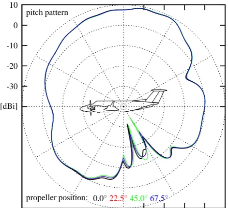
Fig. 2. Simulated pitch pattern of installed VHF top antenna at f=113 MHz.

2 Aircraft model and simulation

As stated above, a numerical simulation of the installed an-tenna performance using the method of moments was ap-plied. In order to obtain the antenna factor, first the gain of the antenna is computed from the radiation pattern. For most of the relevant antennas, equivalent models can be created us-ing analog radiation characteristics, i.e. gainG0of the

origi-nal antenna. For complex antennas with unknown impedance matching networks, the reflection coefficientrcan be deter-mined from measurements.

Effectively, some relevant areas of the platform have ge-ometrical variations within the order of the wavelength or

yaw pattern

67.5◦ 45.0◦

22.5◦

0

-10

-20

-30

[dBi]

Fig. 3. Simulated yaw pattern of installed VHF top antenna at f=113 MHz.

less (propeller blades, leading edge curvatures, surface cur-vatures etc.), so a full-wave solution of Maxwell’s equa-tions is required as opposed to a (less computational inten-sive) asymptotic solution, assuming pure ray-optical behav-ior of the electromagnetic field. For this work a multilevel-fast-multipole accelerated method of moments (MLFMA) is used. The method of moments is a well known and es-tablished technique for antenna analysis (Harrington, 1968), while the MLFMA acceleration is a relative new addition al-lowing the analysis of much larger structures (Chew et al., 2000).

The method of moments requires the geometry to be meshed by elements of about a tenth of the wavelength in size. Here, triangular shaped elements are used. For the aircraft considered here, a Raytheon Beech Super King Air 350, a total of about 16 000 triangles is required to model the geometry at VHF NAV frequencies (108–118 MHz) and of about 600 000 at L-band frequencies around 1 GHz, respec-tively. An image of the VHF mesh is shown in Fig. 1.

Some 3-D-gain antenna patterns referencing an isotropic radiator (G0=1) are exemplified in the following diagrams.

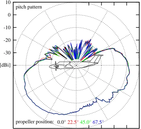
The VHF antenna which is mounted on top of the Beech King Air gives a pitch pattern at 113 MHz shown in Fig. 2 and a corresponding yaw pattern in Fig. 3. In contrast, the concerned L-Band frequencies, e.g. for DME (Distance Mea-suring Equipment), are roughly 10 times higher than for VHF NAV so the resulting pattern has finer structures which can be seen in Figs. 4 and 5 at 1068 MHz. Since the L-band an-tenna is mounted underneath, the aircraft itself shields radi-ation in the upper direction which can be observed in the pitch pattern (Fig. 4). Relevant gain changes due to the

(3)

pitch pattern

67.5◦ 45.0◦

22.5◦

0

-10

-20

-30

[dBi]

Fig. 4. Simulated pitch pattern of installed L-Band (DME) antenna

atf=1068 MHz.

4-blade-propeller position can only be observed at directions which are not relevant for the purpose of the antenna, e.g. to-wards ground as shown in the VHF pitch pattern shown in Fig. 2.

3 Comparison to measurements

In order to verify the simulation results, near field measure-ments of three different antennas were performed by the Physikalisch-Technische Bundesanstalt (PTB) at the airport in Braunschweig. Two of the antennas were dipole antennas for the VHF (108–118 MHz) and UHF (329–335 MHz) band installed above the cockpit whereas the third was a L-band antenna installed underneath the hull of the aircraft.

For the measurements the aircraft was positioned on a 20 m·20 m ground plane made up of a conductive textile. The reference antenna was positioned on a circular arc with a ra-dius ofR=7.75 m facing the aircraft under an aspect angle

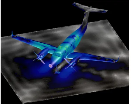
α, as indicated in Fig. 6, between−60 and +60 degrees. The measurements for the L-band antenna were performed in a plane 90 cm above ground, whereas the measurements for the UHF and VHF antennas were performed in planes at three different heights 1.5, 2.5, and 3.5 m above ground. A pho-tograph of the aircraft mounted on pillars above the ground plane and of the reference antenna mast is shown in Fig. 7. The ground plane acts as a co-radiator and therefore has sur-face currents which are visualized exemplarily at 118 MHz in Fig. 8.

yaw pattern

67.5◦ 45.0◦

22.5◦

0

-10

-20

-30

[dBi]

Fig. 5. Simulated yaw pattern of installed L-Band (DME) antenna

atf=1068 MHz.

J. Bredemeyer, T. Kleine-Ostmann, T. Schrader, K. M¨unter and J. Ritter: Airborne Field Strength Monitoring

3 pitch pattern

67.5

◦

45.0

◦

22.5

◦

0.0

◦

propeller position:

10

0 -10

-20

-30

[dBi]

Fig. 4. Simulated pitch pattern of installed L-Band (DME) antenna

at

f

= 1068

_MHz.

yaw pattern

67.5

◦

45.0

◦

22.5

◦

0.0

◦

propeller position:

10

0 -10

-20

-30

[dBi]

Fig. 5. Simulated yaw pattern of installed L-Band (DME) antenna

at

f

= 1068

_MHz.

3 Comparison to measurements

In order to verify the simulation results, near field

measure-ments of three different antennas were performed by the

Physikalisch-Technische Bundesanstalt (PTB) at the airport

in Braunschweig. Two of the antennas were dipole antennas

for the VHF (108-118 MHz) and UHF (329-335 MHz) band

installed above the cockpit whereas the third was a L-band

antenna installed underneath the hull of the aircraft.

For the measurements the aircraft was positioned on a

R

α

Fig. 6. Aspect angle

a radius of

R

= 7

.

75 m facing the aircraft under an aspect

an-gle

α, as indicated in Figure 6, between -60 and +60 degrees.

The measurements for the L-band antenna were performed

in a plane 90 cm above ground, whereas the measurements

for the UHF and VHF antennas were performed in planes

at three different heights 1.5, 2.5, and 3.5 m above ground.

A photograph of the aircraft mounted on pillars above the

ground plane and of the reference antenna mast is shown in

Figure 7. The ground plane acts as a co-radiator and

there-fore has surface currents which are visualized exemplarily at

118 MHz in Figure 8.

Fig. 7. Flight inspection aircraft and reference antenna mast

posi-tioned on a conductive textile ground plane.

3.1 Quantity for comparison

As quantity for the comparison we use the electrical field

strength at the position of the reference antenna which has to

be derived from the detected power

P

d

. This power is a

quan-Fig. 6. Aspect angle.

3.1 Quantity for comparison

As quantity for the comparison we use the electrical field strength at the position of the reference antenna which has to be derived from the detected powerPd. This power is a

qutity integrated over the effective aperture of the reference an-tenna. In order to be able to assign a detector field strength to a discrete point in space its value has to be sufficiently constant in an area comparable to the effective aperture.

If the range between transmission (aircraft) antenna and receiver (reference) antenna is considered as 2-port where

(4)

Fig. 7. Flight inspection aircraft and reference antenna mast

posi-tioned on a conductive textile ground plane.

port 1 is the transmitting antenna and port 2 is the receiving antenna, the scattering parameterS21 describes the relation

between detected power and feed power of the transmitting antennaPf as

Pd = |S21|2Pf . (6)

Substituting the feed powerPf with the expression for the

radiated power

Pt =(1− |S11|2) e−2αlPf , (7)

where the first factor on the right side expresses the mismatch losses and the second factor the losses of the antenna cable with lengthland attenuation coefficientαyields

Pd =

|S21|2

(1− |S11|2)e−2αl

Pt . (8)

The received power can be expressed as the product of ra-diation density in far field approximationS=|E|2/η0

(free-space impedanceη0) and the effective aperture of the receiver

antennaAr by

Pd =SAr =

|E|2

η0

gr λ2

4π (9)

wheregr is the known reference antenna gain.

Using Eq. (8) the magnitude of the electric field strength |E|at the location of the detector antenna can be calculated as

|E|2= |S21|

2

(1− |S11|2)e−2γl

4π·η0

λ2_g r

Pt (10)

with known radiated powerPt and gaingr of the detector

antenna. The feed power is set to 1 Watt to be able to com-pare the measurements to the simulations which have been performed for this power level.

Fig. 8. Surface currents caused by the VHF NAV top antenna above

a ground plane atf=118 MHz. The weakest currents are colored white.

3.2 VHF antenna

The horizontally polarized V-shaped VHF dipole is located above the cockpit. According to its specifications it has a VSWR of 3:1 which corresponds to a reflection factor of |S11|=0.5 (so mismatch loss is 1.25 dB). The RG-400

an-tenna cable has a length of 4.68 m and an attenuation of 0.73 dB in the frequency range from 108 to 118 MHz accord-ing to its specifications.

A fundamental reason for the discrepancy between simu-lation and measurement can be found in the inhomogeneity of the electromagnetic field at the location of the detector antenna. As already discussed in Sect. 3.1, a homogeneous field is the prerequisite for calculating the field strength level from the measured receiver power. Figure 9 shows the real part of the normal component of the radiation power den-sity in comparison to the radiation power denden-sity obtained from the copolar electric field strength over the aspect angle at a height of 3.5 m andf=108 MHz. Obviously the assump-tion of a plane wave with=|E|2/η0is no longer valid which

means that a precise calculation of the field strength from the received power is no longer possible.

For an estimate of the resulting error we simulate the mea-surement situation with a 60 cm dipole at 108 MHz at a height of 3.5 m. The dipole length is comparable to the dimensions of the actual measurement antenna. From the calculated re-ceiver power the field strength is then determined: The dipole has an input impedance ofZD=(9.4− 649.6) and a gain

of 1.84 dBi in free space. In the case of a matched load resistance of ZL=Z_D∗=(9.4+ 649.6) the field strength

level determined in this way is only 0.13 dB below the directly simulated value without antenna. A mismatch in this impedance range has significant impact on the received power and hence on the field strength level. A load resistance

(5)

|ECo|2/η0

Sr

aspect angle /◦

S mW/ m 2 80 60 40 20 0 -20 -40 -60 -80 2.5 2 1.5 1 0.5 0

Fig. 9. Real part of the Poynting vector compared to the

correspond-ing value derived from the copolar electric field strength.

VHF-UHF Antenna f/MHz Gain / dBi 1000 900 800 700 600 500 400 300 200 100 0 5 0 -5 -10 -15 -20 -25

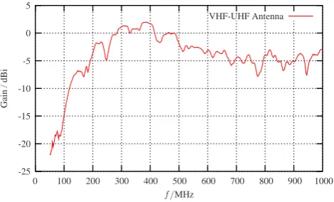
Fig. 10. Gain of the PTB reference antenna.

ofZ_L0=(9.82+ 682) with both real and imaginary values only 5% above the matching value causes the field strength level to decrease by 6 dB.

The reason for this sensitivity can be found in the un-balanced magnitude of real and imaginary part of the in-put impedance of the dipole. We assume that discrepancies between simulations and measurements can be attributed to such a situation. Figure 10 shows the measured gain of the receiver antenna over frequency. It decreases rapidly towards lower frequencies.

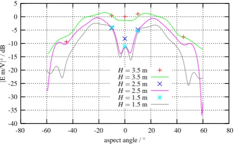
In order to be able to better match simulations and mea-surements, the measured values have been corrected by a constant offset of 2 dB. Figures 11 and 12 show the cor-rected measurements (dots) and the simulations (lines) for 113 and 118 MHz at different receiver antenna heights, re-spectively. For a height of 2.5 m a pronounced dip for a low aspect angle can be observed for both frequencies. We at-tribute this to the influence of the conducting ground plane. Although both simulations and measurements show this be-havior, we observe the strongest discrepancy in this case, es-pecially at 118 MHz. However, with respect to the deviations from the homogeneity of the field and the ideal conduction of the ground used in the calculations, the match between simulations and measurements is satisfactory.

H=1.5 m H=1.5 m H=2.5 m H=2.5 m H=3.5 m H=3.5 m

aspect angle /◦ aspect angle /◦

| E m/V | 2/d B 80 60 40 20 0 -20 -40 -60 -80 5 0 -5 -10 -15 -20 -25 -30 -35 -40

Fig. 11. Field strength level over aspect angle for different

refer-ence antenna heights atf=113 MHz (VHF NAV top antenna, lines: simulation).

H=1.5 m H=1.5 m H=2.5 m H=2.5 m H=3.5 m H=3.5 m

aspect angle /◦

| E m/V | 2/d B 80 60 40 20 0 -20 -40 -60 -80 5 0 -5 -10 -15 -20 -25 -30 -35 -40

Fig. 12. Field strength level over aspect angle for different reference

antenna heights atf=118 MHz (VHF NAV top antenna).

3.3 UHF glideslope antenna

The horizontally polarized UHF dipole is located in front of the V-shaped VHF dipole. According to specifications it has a VSWR of 2:1, corresponding to a reflection factor of |S11|=1/3(=−ˆ 9.5 dB, mismatch loss 0.5 dB). The antenna

is also fed via a RG-400 cable with a length of 5.12 m and a resulting attenuation of 1.5 dB at a frequency of 332 MHz (according to data sheet).

Figure 13 shows the comparison between measurements (dots) and simulations (lines) for the transmitting UHF an-tenna. The agreement is much better in this case because the receiver antenna operates under much better far field con-ditions. Expressed in wavelengths, it is located at approxi-mately three times the distance from the transmitting antenna compared to the previous VHF measurement.

3.4 L-band antenna

The L-band antenna is a monopole. It is fixed underneath the hull of the aircraft between the wings and is vertically

(6)

H=1.5 m H=1.5 m H=2.5 m H=2.5 m H=3.5 m H=3.5 m

aspect angle /◦

|

E

m/V

|

2/d

B

80 60 40 20 0 -20 -40 -60 -80 5

0

-5

-10

-15

-20

-25

-30

-35

-40

Fig. 13. Field strength level over aspect angle at different reference

antenna heights atf=332 MHz (UHF Glideslope top antenna).

polarized. According to specifications it has a VSWR of ap-proximately 1.5:1 which corresponds to a reflection factor of |S11|=0.2(=−ˆ 14 dB, mismatch loss 0.18 dB). The

attenua-tion of the feeding cable is yet unknown.

Figure 14 shows the calculated and measured field strength levels plotted over aspect angle at a frequency of 1075 MHz and at a height ofH=90 cm over ground.

Over a vast range of aspect angles the field strength level difference between measurements and simulations reaches up to 10 dB. Due to the restricted number of measurement points the measurement characteristics lack from under-sampling which makes it more difficult to interpret the curve characteristics. However, over small aspect angle ranges the measurements show a different trend than the simulations. A constant field strength level offset as expected from the con-tribution of the antenna cable attenuation which has not been considered here, would not give a satisfactory explanation.

In order to be able to evaluate the stability of the simu-lated model also in this case the modelling of the transition between wings and hull has been examined further. This area is close to the radiating aircraft antenna and partially non-conducting. Also the influence of the field inhomogene-ity at the location of the reference antenna has been exam-ined. This involved modelling the measurement situation where the receiver dipole, which has a size comparable to the aircraft antenna, was placed at the front aspect. The field strength level has then been calculated from the received power at the receiver antenna according to Eq. (10) and was compared to the directly determined field strength level, af-terwards.

Although the field strength level calculated in this way varies with detector antenna height by 2.5 dB in this case, the field strength level calculated from the receiver powerPr

and the directly determined value differ by less than 0.1 dB atH=90 cm over ground. Therefore the field inhomogene-ity can be excluded as a possible reason for the difference between measurement and simulations.

computation measurement g1

aspect angle /◦

|

E

m/V

|

2/d

B

80 60 40 20 0 -20 -40 -60 -80 12

10

8

6

4

2

0

-2

-4

-6

Fig. 14. Field strength level at 90 cm reference antenna height over

aspect angle atf=1075 MHz.

A possible explanation for the difference between mea-surements and simulations could be found in the realization of the conducting ground plane. The reflection character-istics of the conducting textile remains to be determined in an adequate measurement setup for both polarization types. Also the local variation in flatness of the ground plane (as can be seen in Fig. 7) is not negligible.

3.5 Mutual L-band S-parameters

In addition to the ground plane measurements between an aircraft antenna and a remote detector antenna in-flight mea-surements between mutual aircraft L-band antennas under-neath the hull were performed. In order to further verify the accuracy of the computer model, three pairs of antennas were measured. The amplitude of transmission factors|S21|

were compared to simulated data obtained from the MLFMA model of the aircraft for the respective antennas.

The measurements have been performed during an 1 h test flight over Northern Germany using a HP8753D vector net-work analyzer. The measurements were performed at an al-titude of 5000 ft. with a cloud ceiling far underneath and above the aircraft. The transponder was switched off to pre-vent unwanted interference with the measurements. After TOSM calibration of the vector network analyzer at the end of the two 2.5 m long measurement cables and after the con-secutive measurements of the antennas under test the perfor-mance of the network analyzer was checked based on the

Encriterium (EAL, 1996). Measurements of calibrated PTB

precision attenuators (10 dB, 20 dB, 30 dB and 50 dB) proved that the antenna measurements in between are within the ex-pected measurement uncertainty of less than 0.25 dB.

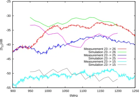
Figure 15 shows the result of the measurements between the previously described L-band antenna centered between the wings used as transmission antenna (no. 23 in numera-tion of all aircraft antennas) and three other L-band antennas used as detector antennas (no. 26 underneath the right wing, no. 25 underneath the left wing and antenna 15 underneath

(7)

-55 -50 -45 -40 -35 -30 -25

900 950 1000 1050 1100 1150 1200 1250 |S21

|/dB

f/MHz

Measurement 23 -> 26 Simulation 23 -> 26 Measurement 23 -> 25 Simulation 23 -> 25 Measurement 23 -> 15 Simulation 23 -> 15

Fig. 15. Comparison of simulated and measured S-parameters of

L-band antennas. The numbers 15, 23, 26 according to list of all aircraft antennas.

the rear hull). Measurements and calculations agree well in all cases but especially for the antenna pairs 23–25 and 23– 15. The calculated attenuation has the tendency to be weaker than the measured values. We attribute this to the attenuation of several meters of RF cable which have been neglected so far. Further investigations to incorporate cable attenuation measurements into the calculation of effective antenna fac-tors are underway.

4 Conclusions

We showed that a balanced combination of antenna measure-ments, platform modelling and MoM simulations is the key to obtain the effective antenna installed performance. How-ever, some problems impede the comparison of measurement results and numerical solutions under certain circumstances: The VHF results were gained in a near field environment whereas the L-band antennas underneath the aircraft did not meet the ideal conditions above the ground plane as taken for granted in the model. In the VHF case one has to con-sider alternative measurement concepts. A solution could be to implement a near field scanner in context with adequate near to far field transformations. Further work is needed to implement such technologies and the authors will continue their work in upcoming projects.

Acknowledgements. The authors would like to thank M.

Schwen-dener and J. Follop of Flight Calibration Services for their assis-tance during the measurement campaigns and J. Reiter of EADS for his contributions to the simulations.

References

Balanis, C. A.: Antenna Theory Analysis and Design, Wiley, New York, 1997.

Bredemeyer, J., Battermann, S., Garbe, H., and Ritter, J.: Antenna Installed Performance of a Flight Inspection Aircraft, Proceed-ings of International Symposium on Precision Approach and Au-tomatic Landing (ISPA 2004), Munich, Germany, 2004. Chew, W. C., Jin, J.-M., Michielssen, E., and Song, J. M.: Fast and

efficient algorithms in computational electromagnetics, Artech House, Boston, London, 2000.

DIN EN 45003 (Akkreditierungssysteme für Kalibrier- und Prüflaboratorien; allgemeine Anforderungen für Betrieb und An-erkennung), 1995.

International Civil Aviation Organization: DOC 8071, Manual on Testing of Radio Navigation Aids, Volume I: Testing of Ground-based Radio Navigation Systems, Montreal, 2000.

European cooperation for Accreditation of Laboratories, Publica-tion Reference EAL-P7, EAL Interlaboratory Comparisons, Edi-tion 1, March, 1996.

Harrington, R. F.: Field Computation by Moment Methods, Cazen-ovia, N.Y., USA, 1968.

Kraus, J. D.: Antennas, Mc-Graw-Hill, Boston, 1988.

Unger, H.-G.: Elektromagnetische Wellen auf Leitungen, 4. Aufl., Heidelberg, 1996.