Some robust integrators for large time dynamics

(1)

Razafindralandy et al.Adv. Model. and Simul. in Eng. Sci. (2019) 6:5

https://doi.org/10.1186/s40323-019-0130-2

R E V I E W

Open Access

Some robust integrators for large time

dynamics

Dina Razaﬁndralandy

1*

, Vladimir Salnikov

2

, Aziz Hamdouni

1

and Ahmad Deeb

1

*_{Correspondence:}

dina.razaﬁ[email protected]

1_{Laboratoire des Sciences de}

l’Ingénieur pour l’Environnement (LaSIE), UMR 7356 CNRS, Université de La Rochelle, Avenue Michel Crépeau, 17042 La Rochelle Cedex, France Full list of author information is available at the end of the article

Abstract

This article reviews some integrators particularly suitable for the numerical resolution of diﬀerential equations on a large time interval. Symplectic integrators are presented. Their stability on exponentially large time is shown through numerical examples. Next, Dirac integrators for constrained systems are exposed. An application on chaotic dynamics is presented. Lastly, for systems having no exploitable geometric structure, the Borel–Laplace integrator is presented. Numerical experiments on Hamiltonian and non-Hamiltonian systems are carried out, as well as on a partial diﬀerential equation. Keywords: Symplectic integrators, Dirac integrators, Long-time stability, Borel summation, Divergent series

Introduction

In many domains of mechanics, simulations over a large time interval are crucial. This is, for instance, the case in molecular dynamics, in weather forecast or in astronomy. While many time integrators are available in literature, only few of them are suitable for large time simulations. Indeed, many numerical schemes fail to correctly predict the expected physical phenomena such as energy preservation, as the simulation time grows.

For equations having an underlying geometric structure (Hamiltonian systems, varia-tional problems, Lie symmetry group, Dirac structure,. . .), geometric integrators appear to be very robust for large time simulation. These integrators mimic the geometric struc-ture of the equation at the discrete scale.

The aim of this paper is to make a review of some time integrators which are suitable for large time simulations. We consider not only equations having a geometric structure but also more general equations. We ﬁrst present symplectic integrators for Hamiltonian systems. We show in “Symplectic integrators” section their ability in preserving the Hamil-tonian function and some other integrals of motion. Applications will be on a periodic Toda lattice and onn-body problems. To simplify, the presentation is done in canonical coordinates.

In “Dirac integrators” section, we show how to ﬁt a constrained problem into a Dirac structure. We then detail how to construct a geometric integrator respecting the Dirac structure. The presentation will be simpliﬁed, and the (although very interesting) theo-retical geometry is skipped. References will be given for more in-depth understanding. A

©The Author(s) 2019. This article is distributed under the terms of the Creative Commons Attribution 4.0 International License (http://creativecommons.org/licenses/by/4.0/), which permits unrestricted use, distribution, and reproduction in any medium, provided you give appropriate credit to the original author(s) and the source, provide a link to the Creative Commons license, and indicate if changes were made.

(2)

Razafindralandy et al.Adv. Model. and Simul. in Eng. Sci. (2019) 6:5 Page 2 of 29

numerical experiment, showing the good long time behaviour of Dirac integrators, will be carried out.

In “Borel–Laplace integrator” section, we present the Borel–Padé–Laplace integrator (BPL). BPL is a general-purpose time integrator, based on a time series decomposition of the solution, followed by a resummation to enlarge the validity of the series and then reducing the numerical cost on a large time simulation. Finally, the long time behaviour will be investigated through numerical experiments on Hamiltonian and non-Hamiltonian system, as well as on a partial diﬀerential equation. Numerical cost will be examined when relevant.

Symplectic integrators

We ﬁrst make some reminder on Hamiltonian systems and their ﬂows in canonical coor-dinates. Some examples of symplectic integrators are given afterwards and numerical experiments are presented.

Hamiltonian system

A Hamiltonian system inRd×Rdis a system of diﬀerential equations which can be written as follows: ⎧ ⎪ ⎪ ⎪ ⎪ ⎪ ⎪ ⎨ ⎪ ⎪ ⎪ ⎪ ⎪ ⎪ ⎩ dq dt =

∂H ∂p,

dp dt = −

∂H ∂q,

(1)

the HamiltonianHbeing a function of time and of the unknown vectorsq=(q1,. . ., qd)T andp=(p1,. . ., pd)T. Equation (1) can be written in a more compact way as follows:

du

dt =J∇H (2)

whereu=(q,p)T,∇H = ∂H

∂u andJis the skew-symmetric matrix

J=

0 I_d

−Id 0

,

Idbeing the identity matrix ofRd.

The ﬂow of the Hamiltonian system (2) at timetis the functiontwhich, to an initial conditionu0associates the solutionu(t) of the system. More precisely,tis deﬁned as:

t:

Rd_×_Rd _−→_Rd_×_Rd

u0₌₍_q0_,_p0₎T_−→_u₍_t₎₌₍_q₍_t₎_,_p₍_t₎₎T_.

(3)

The property thatJ−1=JT= −Jleads to the symplecticity property oft:

(∇t)TJ(∇t)=J. (4)

Note thatJcan be seen as an area form, in the following sense. Ifvandware two vectors ofRd×Rd, with components

v=(vq1,. . ., vqd, vp1,. . ., vpd)

T

, w=(wq1,. . ., wqd, wp1,. . ., wpd)

(3)

then

vT_J_w₌ d

i=1

vqiwpi−vpiwqi

.

In words,vTJwis the sum of the areas formed by vandwin the planes (qi, pi). The symplecticity property (4) then means that the ﬂow of a Hamiltonian system is area preserving.

In the sequel,His assumed autonomous in time. It can then be shown thatHis preserved along trajectories.

Flow of a numerical scheme

Consider a numerical scheme which computes an approximationun_{of the solution}_u₍_tn₎ of Eq. (2) at timetn. The ﬂow of this scheme is deﬁned as

ϕtn:u0=(q0,p0)T −→ un=(qn,pn)T (5)

For a one-step integrator, with a time stept=tn+1−tn(which may depend onn), it is more convenient to work with the one-step ﬂow

ϕn

t:un −→ un+1 (6)

As an example, consider the explicit Euler integration scheme ⎧ ⎪ ⎪ ⎪ ⎪ ⎪ ⎪ ⎨ ⎪ ⎪ ⎪ ⎪ ⎪ ⎪ ⎩

qn+1₌_qn₊_t∂H ∂p(qn,pn)

pn+1₌_pn₋_t∂H

∂q(qn,pn).

The one-step ﬂow of this scheme is

ϕn

t(un)=un+tJ∇H(un). (7)

The one-step ﬂow of a fourth order Runge–Kutta scheme is

ϕn

t(un)=un+t

f1+2f2+2f3+f4

6 (8)

where

f1=J∇H(un), f2=J∇H un+₂tf1

,

f3=J∇H un+₂tf2

, f4=J∇H(un+t f3).

Some symplectic integrators

A time integrator is called symplectic if its ﬂow is symplectic, meaning that

(∇ϕtn)TJ(∇ϕ_tn)=J. (9)

Geometrically, a symplectic integrator is then a time scheme which preserves the area form. For a one-step scheme, this property is equivalent to

(∇ϕn_t)TJ(∇ϕn_t)=J (10)

at each iterationn.

Whend=1, it can easily be shown that, for an explicit Euler scheme,

(∇ϕn_t)TJ(∇ϕn_t)=

1+t2

∂2_H

∂q2

∂2_H

∂p2 −

∂2_H

∂q∂p

(4)

meaning that the explicit Euler scheme is not symplectic. Neither the implicit Euler scheme is symplectic. By contrast, by mixing the explicit and the implicit Euler scheme, we get a symplectic scheme, called symplectic Euler scheme, deﬁned as follows

⎧ ⎪ ⎪ ⎪ ⎪ ⎪ ⎪ ⎨ ⎪ ⎪ ⎪ ⎪ ⎪ ⎪ ⎩

qn+1₌_qn₊_t∂H

∂p(qn,pn+1),

pn+1₌_pn₋_t∂H

∂q(qn,pn+1).

(12)

Note that in (12), one can take (qn+1,pn) in the right-hand-side instead of (qn,pn+1). This leads to the other symplectic Euler scheme.

Both symplectic Euler schemes are ﬁrst order. A way to get a second order scheme is to compose two symplectic Euler schemes with time stepst/2. One then obtains the Störmer–Verlet schemes [13]. Another way is to take the mid-points in the right-hand side of an Euler scheme [15], yielding the mid-point scheme:

⎧ ⎪ ⎪ ⎪ ⎨ ⎪ ⎪ ⎪ ⎩

qn+1₌_qn₊_h_∇

pH

qn+1₂_,_pn+1₂_,

pn+1₌_pn₋_h_∇

qH

qn+1 2_,pn+12

,

(13)

where

qn+1₂ ₌ qn+qn+1

2 , p

n+1₂ ₌ pn+pn+1

2 .

Symplectic Runge–Kutta schemes of higher order can be built as follows. An s-stage Runge–Kutta integrator of Eq. (1) is deﬁned as [14,29]:

Ui=un+t s

j=1

αijJ∇H(Uj), i=1,. . ., s,

un+1₌_un₊_t s

i=1

βiJ∇H(Ui),

(14)

for some real numbersαij,βi,i, j =1,. . ., s. Scheme (14) is symplectic if and only if the coeﬃcients verify the relation [18,28]:

βiβj=βiαij+βjαji, i, j=1,. . ., s. (15)

An example of symplectic Runge–Kutta scheme is the 4th order, 3-stage scheme deﬁned by the coeﬃcients

α= ⎛ ⎜ ⎜ ⎜ ⎜ ⎜ ⎜ ⎜ ⎜ ⎜ ⎝ b

2 0 0

b 1

2−b 0

b 1−2b b 2 ⎞ ⎟ ⎟ ⎟ ⎟ ⎟ ⎟ ⎟ ⎟ ⎟ ⎠

, β =

b 1−2b b

, (16)

where

b= 2+2

1/2₊₂−1/3

(5)

Many other variants of symplectic Runge–Kutta methods can be found in the literature (see for example [10]).

Symplectic integrators do not preserve exactly the Hamiltonian in general. However, the symplecticity condition seems to be strong enough that, experimentally, symplectic integrators exhibit a good behaviour toward the preservation property. In fact, we have the following error estimation on the Hamiltonian [1,12]:

|H(pn, qn)−H(p0, q0)| =O(tr) fornt≤e2γt (17)

for some constantγ >0,rbeing the order of the symplectic scheme. This relation states that the error is bounded over an exponentially long discrete time. Moreover, it was shown in [5] that symplectic Runge–Kutta methods preserve exactly quadratic invariants.

In the next subsection, some interesting numerical properties of symplectic schemes are highlighted through some model problems.

Numerical experiments

Periodic Toda lattice

The evolution of a periodic Toda lattice withdparticles can be described with the Hamil-tonian function

H =

d

k=1

1 2p

2

k+eqk−qk+1

whereqk is the (one-dimensional) position of thek-th particle,qd+1 = q1andpk is its momentum. A periodic Toda lattice is completely integrable and it is known that the eigenvalues of the following matrixLare ﬁrst integrals of the system:

L= ⎛ ⎜ ⎜ ⎜ ⎜ ⎜ ⎜ ⎜ ⎜ ⎜ ⎝

a1b1 0 0 0 · · · 0 bd b1a2b2 0 0 · · · 0 0

0 b2a3 b3 0 · · · 0 0 ..

.

0 0 0 · · ·0bd−2ad−1bd−1 bd 0 0 · · ·0 0 bd−1 ad

⎞ ⎟ ⎟ ⎟ ⎟ ⎟ ⎟ ⎟ ⎟ ⎟ ⎠ (18) where

ak = − 1

2pk, bk = 1 2e

1

2(qk−qk+1)_.

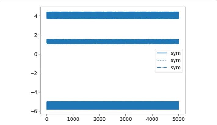
In the numerical test, we considerd=3 particles, positioned initially atq1=0,q2=2 andq3=3. The initial momenta arep1=0.5,p2= −1.5 andp3=1.

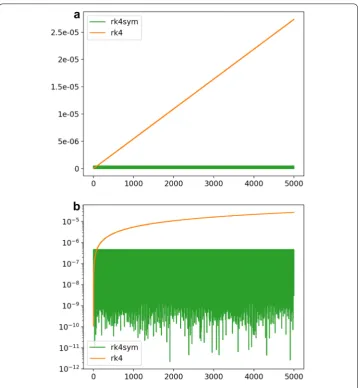
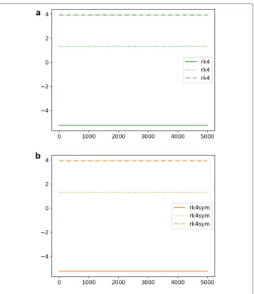
First, we choose a time stept= 10−2. The Hamiltonian equation is solved with the classical 4-th order Runge–Kutta scheme (RK4) and the symplectic version (RK4sym) deﬁned by (16) up tot = 5000. The relative error on the Hamiltonian is presented in Fig.1. As can be seen, the RK4 error oscillates and increases globally linearly. It remains acceptable fort < 5000 since it does not exceed 2.735·10−5_{. The RK4sym error also} oscillates but is much closer to zero. It is bounded by 4.625·10−7, that is an order of 10−2 bellow RK4 error att = 5000, as can be observed in Fig.1b. Figure2shows that both schemes globally preserve the three eigenvalues of the matrixL.

(6)

Fig. 1 Toda lattice. Relative error|H(un)−H(u0)|

|H(u0₎_| witht=10−2in linear scale (a) and in logarithmic scale (b)

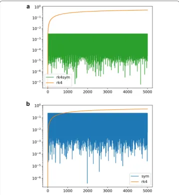
error oscillates around 2.26·10−3but does not present any increasing global tendency. Its highest value is about 3.27·10−3, as can be checked in the ﬁgure.

A comparison between RK4 and the symplectic Euler scheme deﬁned in (12) is also given in Fig.3b. It shows that the error of the Euler scheme oscillates around 0.83·t and does not exceed 2.42t. So, fortgreater than 820, even the ﬁrst order symplectic Euler scheme produces an error smaller than the 4-th order non-symplectic Runge–Kutta scheme on the Hamiltonian.

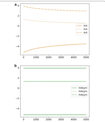
The evolution of the eigenvalues of the matrixLis presented in Fig.4. It clearly shows that the eigenvalues are not preserved by the classical Runge–Kutta scheme. For example, the computed smallest eigenvalue att = 5000 is about−3.50 whereas its initial value is

(7)

Fig. 2 Toda lattice. Evolution of the eigenvalues ofLwitht=10−2_._a_RK4._b_RK4sym

It is clear from these experiments that symplectic schemes are particularly stable for large time simulations, where the user wishes a time step as large as possible to reduce the computation cost. In some situation, even a symplectic scheme with a smaller order gives better results over a long time than a classical integrator.

n-body problem

As a second example, consider the system ofdbodies subjected to mutual gravitational forces. The evolution of the system is described by the Hamiltonian function

H =

d

k=1 1 2

pk2

m_k −

d

k=1 d

l=k+1

Gmkml ql−qk

.

In this expression,qkandpkare the position vector and the momentum of thek−th body, mkis its mass andGis the gravitation constant.

(8)

Fig. 3 Toda lattice. Relative error onHwitht=10−1_._a_{RK4 and RK4sym.}_b_{RK4 and Symplectic Euler}

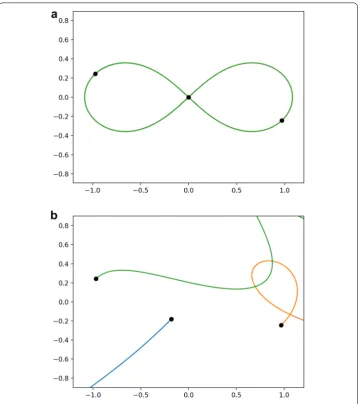
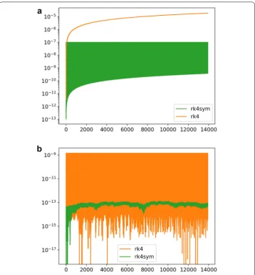
T 6.32591398. The common trajectory and the initial position are presented in Fig.6a. The simulation is run up tot=2200T, with a time stept=0.02T. In these conﬁgura-tions, the classical Runge–Kutta scheme provides a fairly good result but the symplectic scheme is much more accurate regarding the preservation properties. The relative error of RK4 on the Hamiltonian increases linearly and is about 1.87·10−5at the ﬁnal time. It can be viewed in Fig.7a in logarithmic scale. The relative error of RK4sym onHoscillates but never exceeds 9.99·10−8. The errors on the angular momentum are plotted in Fig.7b. It shows that the error of RK4 is bounded by 1.4·10−9whereas the error of RK4sym is remains under the machine precision (around 2·10−12_).

(9)

Fig. 4 Toda lattice. Evolution of the eigenvalues of_Lwith_t₌10−1_._a_RK4._b_RK4sym

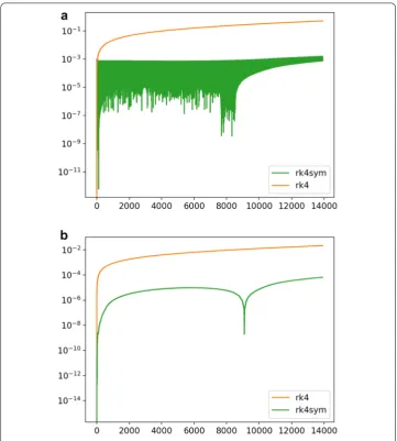
this time value, the error on the Hamiltonian with the symplectic RK4 is about 7.75·10−4. It reaches 1 percent much later, aroundt6315·T 39950 (not seen on the graphic). These numerical experiments show again that symplectic schemes are more robust than classical ones for long time dynamics simulation. They have a good behaviour regarding the preservation of the Hamiltonian and some other ﬁrst integrals despite the perturbation introduced in the initial conﬁguration. Similar results have been obtained in a previous work [24] on an harmonic oscillator, on Kepler’s problem and on vortex dynamics.

Obviously, not all mechanical systems ﬁt into the Hamiltonian formalism, hence there are other geometric constructions that are worth being considered in the context of structure-preserving integrators.

Dirac integrators

(10)

Fig. 5 Toda lattice. Evolution of the eigenvalues ofLwith the symplectic Euler scheme andt=10−1

Originally, Dirac structures appear in the work of Courant [6]. The initial motivation was coming from mechanics. As is known, for mechanical systems one can choose between Lagrangian and Hamiltonian formalisms, both being equivalent in ﬁnite dimension. The rough idea behind Dirac structures is to consider both formalisms simultaneously, i.e. working with velocitiesandmomenta, however not forgetting that those are dependent variables. Geometrically, this means that instead of choosing between the tangent and cotangent bundlesTMorT∗Mfor the phase space, we consider their direct sumE = TM⊕T∗Mand a subbundle of it, subject to some compatibility conditions. Somehow, the original work did not have direct applications to mechanics, since the geometry of the problem turned out to be rather intricate, and gave rise to a lot of development inhigher structuresand intheoretical physics. In the last decade, however, it was revived with the introduction of so-called port–Hamiltonian [32] and implicit Lagrangian systems [33,34].

Geometric construction

Not to overload the presentation here with geometric details, let us talk about spaces instead of bundles. To recover the geometric picture, a motivated reader is invited to read the original paper [6] of Courant or the overview of relevant results in [27]. The object of study will beR2d(in the same notations as in the beginning of the previous section), and some natural construction around it. We are going to view it asR2d = Rd×V∗, that is the trivial bundle overRdwith a ﬁber beingV∗—the dual of somed-dimensional vector spaceV. Morally,Vis the space of velocitiesvat each pointqandV∗corresponds to the space of momentap. In coordinates:

q=(q1,. . ., qd)T∈Rd, v=(v1,. . ., vd)T ∈V, p=(p1,. . ., pd)T ∈V∗.

(11)

Fig. 6 Three-body problem. Figure-eight orbit (a) and perturbed (b) initial positions and trajectories

And since everything depends on the pointq, globally, the permitted vector ﬁeldsv(q) live in the kernel⊂Rd×V ofmdiﬀerential 1-formsαa(q), a=1,. . ., m.

To transfer this construction fromRd×V toRd×V∗, one needs to consider double vector bundles [31]. In our simpliﬁed setting this means that the space of interest is V =R4d_{, where each component has some geometric interpretation. Namely, we consider} Vas the tangent toRd_×_V∗_{. Naturally,}_Rd_×_V_{is embedded in}_V_{(recall that}_V_{is tangent to} Rd_{). The constraint set is then a subset ˜}_⊂_V_{, and the diﬀerential forms}_αa₍_q_{) generate its} annihilator0that naturally belongs toV∗. Note that, sinceRd×V∗is a symplectic space, it is equipped with a bilinear antisymmetric non-degenerate closed form (this form is the generalisation of the matrixJof “Symplectic integrators” section in non-canonical coordinates). One can then construct a symplectic mapping :V→V∗.

We can now deﬁne theDirac structure1associated to the system with constraints:

(12)

Fig. 7 Eight-orbit conﬁguration. Error on the Hamiltonian (a) and on the angular momentum (b)

D= {(w,β)∈V×V∗|w∈˜, β− w∈0}.

To define the dynamics of the system, we introduce two more objects. First, the Lagrangian, which as usual is a mappingL:Rd×V →R, induces its differential which is a mappingdLfromRd×Vto its cotangent. And again by post-composing it with a sym-plectomorphism of the appropriate double bundles, one constructs theDirac differential which locally reads

DL:

Rd_×_V _−→_V∗

(q,v)−→

q, ∂L ∂v, −

∂L ∂q, v

Second, the evolution of the system will be described by a so-calledpartial vector ﬁeld X, i.e. a mapping

X : ⊕Leg() ⊂

(13)

Fig. 8 Perturbed conﬁguration. Error on the Hamiltonian (a) and on the angular momentum (b)

where Leg() is the image ofby the Legendre transform. X should be viewed as a vector ﬁeld onRd×V∗, with the momenta parametrized by the Legendre transform of the velocities compatible with the constraints.

With the above notations, theimplicit Lagrangian systemis a triple (L,, X), such that (X,DL)∈D. In local coordinates, this means:

⎧ ⎪ ⎪ ⎪ ⎨ ⎪ ⎪ ⎪ ⎩

dq

dt ∈, p= ∂L ∂v,

dq dt =v,

dp dt −

∂L ∂q ∈0.

(19)

One understands easily the mechanical interpretation of the ﬁrst three equations above. The forth one can be rewritten as

dp dt −

∂L ∂q =

m

a=1

λaαa,

(14)

Discretization

It is important to note that the previous section is not just a “fancy” way of recovering the well-known theory: every step of the construction admits a discrete analog. We brieﬂy present the recipe of this discretization and, again, refer the interested reader to [27] for details and examples.

The system is characterized by the following continuous data: the Lagrangian function L(q,q˙) and the set of constraint 1-formsαa, a=1,. . ., m. The discrete versionL_dof the Lagrangian at timetn_is

Ld =t L(qn,vn).

And the constraints are rewritten as

< αa

d,vn>=0, a=1,. . ., m.

where< α_da,vn>=αa_d(vn), andαa_dis a discrete version ofαa. In the Equations above,qn is the value ofqandvnis an approximation of the velocityv, both at timetn.

To construct the numerical method out of these data, one applies the following proce-dure:

pn+1₌ 1

t ∂L_d

∂vn (20)

pn₋ 1 t

∂Ld ∂vn +

∂Ld ∂qn =

m

a=1

λa∂ < α a d,vn>

∂vn (21)

< αa

d,vn>=0, a=1,. . ., m. (22)

The variables appearing explicitly are the values ofpat then-th and the (n+1)-st steps, andvn should be some approximation of the velocity, thus bringingqn to the system. Here, we consider two natural options:

• vn:= q

n+1₋_qn

t , we label it Dirac-1, and

• vn:= q

n+1₋_qn−1

2t , labelled Dirac-2.

Dirac-1 permits to recover the method from [19] whereas we introduced Dirac-2 in [27]. In both cases, we obtain 2d+mequations:dfrom each of the lines (20) and (21) of the equations above, andmfrom the constraints (22). At then-th step the unknowns areqn+1,

pn+1_and_λ₌₍_λ

1,. . .,λm), so the system we obtain is complete. It is linear inλandpn+1, and when the constraints are holonomic, inqn+1as well.

It is important to note that, in some sense, this construction generalizes the previous section. If one considers the system without constraints but still applies the procedure, (22) becomes obsolete, and in (21) the right-hand-sides vanish, so one obtains a numerical method for the dynamics of a Lagrangian system governed by L. By a straightforward computation, one checks that for a natural mechanical system with a potentialU, i.e. whenL = 1₂mv2₊_U₍_q_{), Dirac-1 is symplectic. And it is also meaningful to consider a} symplectic version of Dirac-2 (we do not detail it here since we would need to explain what is symplecticity for a multistep method).

Example: chaos for double pendulum

(15)

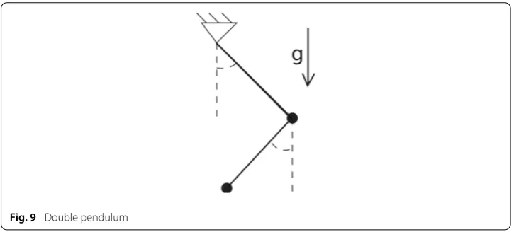
Fig. 9 Double pendulum

to rigid inextensible weightless rods (see Fig.9). Although, it looks like a classical well-studied problem, it is a bit challenging for simulations. In the absence of the gravity ﬁeld, this is a textbook example of an integrable system (energy and angular momentum are conserved, thus the Liouville–Arnold theorem can be applied). With the gravity, the “folkloric knowledge” says that it is chaotic, although as far as we know there is no rigorous proof of the fact. For the integrability, there is a semi-numerical proof of absence of an additional ﬁrst integral in [26], using the computation of the monodromy group by a method presented in [25]. Anyway, the apparent chaoticity of the system results in its sensitivity to parameters and initial data in the numerical simulation.

From the point of view of the previous subsection, this is a typical example of a system with constraints: the distance1from the ﬁrst mass point to the origin and the distance

2between the two mass points are ﬁxed. The system admits a parametrization in terms of angles, but we will pretend not to know it, to test the method.

We thus consider a mechanical system of two mass points given by the Lagrangian

L(q1,q2,q˙1,q˙2)= 1 2m1q˙1

2₊1 2m2q˙2

2₋_m

1gq1,y−m2gq2,y,

subject to the constraints

ϕ1_≡_q

12−21=0, ϕ2≡ q2−q12−22=0.

To recover the framework of the numerical method given by (20–22), we take αa ≡ dϕa, a=1,2.

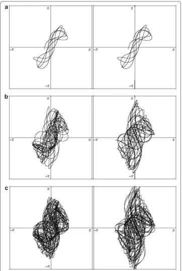
The typical result of simulations is shown in Fig.10. Dirac-2 and explicit Euler methods are compared. For visualization (but not for computation), we use the angle representation of the double pendulum (see Fig.9). Both algorithms start with the same initial data, and the same timestept =0.0001. They are in good agreement in the beginning as can be seen on the two top-graphics of Fig.10. But already at timeT =50, the diﬀerence is visible (graphics in the middle). And towardsT =100 the diﬀerence becomes dramatic: for the Euler method the pendulum is making full turns instead of oscillation. And this is clearly a computation artifact, since decreasing the timestep one gets rid of the discrepancy and recovers the left picture for both methods. Note also that Dirac structure based method preserves the constraints much better than the Euler one: the error is 2.2·10−6compared to 0.06 respectively.

(16)

Fig. 10 Double pendulum: Comparison of dynamics. Left: Dirac-2, right: explicit Euler. Region swept by the trajectory untilaT=10,bT=50 andcT=100

structure based methods: the Lagrange multipliers are treated like other dynamical vari-ables, there is no need to resolve “by hand” the equation related to constraints (22).

(17)

to more robust numerical schemes. In the last section, we propose an integrator which is suitable to general systems where no geometric structure is exploitable for numerical simulations.

Borel–Laplace integrator

Consider an ordinary diﬀerential or a semi-discretized partial diﬀerential equation:

du

dt =F(u(t), t) (23)

associated to an initial conditionu(t=0)=u0. We look for a time series solution:

˘ u(t)=

+∞

n=0

untn. (24)

Generally, the right-hand side of (23) can be expanded into

F(u(t), t)=

+∞

n=0

Fn(u0,. . ., un)tn (25)

whereFnis then-th Taylor expansion of the functionF(u(t), t) att = 0. Injecting (24) and (25) into Eq. (23) leads to the following recurrence relation

(n+1)un+1=Fn(u0,. . ., un) for alln∈N. (26) This relation enables to compute the terms of the series ˘u. See also sections and for concrete examples. A Borel summation is then applied to series (24). This summation is essential if the convergence radius of the series is zero and the series is summable [2,20]. If the convergence radius is not zero, the Borel summation enlarges the domain of validity of the series.

The Borel sum of ˘u(t) is

Su˘(t)=[L◦P◦B]˘u(t) (27)

whereBis the Borel transform,P is a prolongation along a semi-line inClinking 0 to inﬁnity (we will take the real positive semi-line), andLis the Laplace transform along this semi-line. The theory of Borel summation can be found, for example, in [2,20–22]. Some other works on BPL, as a time integrator, can be found in [8,23]. In this section, we present very brieﬂy the Borel-Padé-Laplace algorithm, integrated into a numerical scheme.

The Borel-Padé-Laplace summation integrator (BPL) consists in the following steps:

• Given an initial conditionu(t0)=u0, compute a truncated series solution via

recur-rence (26): ˘uN(t)=N n=0unt

n_.

• Compute its Borel transform:Bu˘N(ξ)=N−1 n=0

un+1 n! ξ

n_.

• Transform Bu˘N(ξ) into a rational fraction function via a Padé approximation:

PN(ξ)= a0+a1t+. . .aNnumtNnum

b0+b1t+. . .bNdentNden

The Padé approximation materializes the prolongation in the Borel summation pro-cedure.

• Apply a Laplace transformation (at 1/t) onP(ξ) to obtain a numerical Borel sum Su˘N(t)=

_+∞

0

PN(ξ)e−ξ/tdξ.

(18)

• TakeSu˘N(t) as an approximate solutionu(t) of (23) within the integral [t0, t1] where the residue of the equation is smaller than a parameterres.

• Restart the algorithm withu0 =u(t1) as initial condition to obtain an approximate solution for larger values oft.

At each iteration,t1−t0is considered as the (adaptative) time-step of the scheme. The average time-step will be used for comparisons in numerical experiments. Note that at each time, the approximate solution has an analytical representation as a Laplace integral. A continued fraction representation can also be used [9].

An advantage of BPL is that it is totally explicit, in contrast with symplectic integrators in general. Moreover, changing the order of the scheme is as easy as settingNto a diﬀerent value. Note also that the resummation procedure can be done componentwise, enabling an easy parallelization on multi-core computers. However, no such optimization has been done in the present article.

In the following subsection, a partial analysis of the symplecticity property of BPL is presented.

High-order symplecticity

The numerical ﬂow of BPL can be deﬁned as

u0 → Su˘N(t).

Currently, no symplecticity result has yet been found on this scheme. Instead, it can be shown that a scheme based on the truncated series ˘uwithout the resummation procedure is symplectic at orderN, if the equation is symplectic.

The ﬂow of the scheme based on the time series ˘uis

ϕt,u˘ : u0 → u˘(t)=

+∞

n=0 tnun.

Lemma 1 The ﬂow of the scheme based on the time series, applied to the Hamiltonian Eq. (2) is

ϕt,u˘ =

+∞

n=0 tn n!JD

n_∇_H _{where D}n₌ dn−1

dtn−1 (28)

agreeing that D0=1.

This can be straightforwardly deduced by injecting the time series ˘uin (2) and identifying the coeﬃcients of eachtn. Next, if the series is convergent then, inside the convergence disc, ˘uis the exact solution. In this case, ˘ϕtis symplectic. We reformulate this statement in the following theorem.

Theorem 2 If the series is convergent then

(∇ϕt,u˘)TJϕt,u˘ =J. (29)

Corollary 3 If the series is convergent then, for any n≥1, n

k=0 1 k!

1 (n−k)!(JD

k_∇_H₎T_J_(J

(19)

This corollary is obtained by injecting the series development (28) into (29) and identifying the coeﬃcients oftnforn≥1. Forn=0, we simply have

(J∇H)TJ(J∇H)=J. (31)

When the series is truncated at orderN, the ﬂow of ˘uNis

ϕt,u˘N : u0 → u˘N(t)= N

n=0 tnun.

The following theorem shows that the scheme based on the truncated series is symplectic at orderN+1.

Theorem 4 If the series is convergent then

(∇ϕ_t,_u_˘N)TJ∇ϕ_t,_u_˘N =J + O(tN+1) (32)

for t∈[0,δt]whereδt is the convergence radius.

Indeed,

(∇ϕ_t,_u_˘N)TJ∇ϕ_t,_u_˘N =

N

n=0 n

k=0 tn k!(n−k)!(JD

k_∇_H₎T_J₍_J_Dn−k_∇_H₎

+

2N

n=N+1 N

k=n−N tn k!(n−k)!(JD

k_∇_H₎T_J₍_J_Dn−k_∇_H₎_.

Using (30) and (31), the theorem follows. Note that in Theorem4,δtis generally small. In the following subsections, BPL is implemented and tested on a Hamiltonian equation. Next, we present some experiments on non-Hamiltonian equations.

In simulations, the truncation order of the series is set toN=10 unless otherwise stated. The degree of the numerator and the denominator of the Padé approximant areNnum=4 andNden=5. A singular value decomposition is used to strengthen the robustness of the Padé calculation [11]. Twenty Gauss–Laguerre roots are used for the quadrature.

The aim of these simulations is not to make an extensive comparison of BPL with classical schemes (this will be done in a forthcoming paper) but only to show the potential of the scheme in predicting long time dynamics.

Periodic Toda lattice

We consider again the periodic Toda lattice from “Periodic Toda lattice” section. The quality parameterresof BPL is choosen such that the mean time stepδtis approximately 0.1, and compare the results with that of RK4 and RK4sym (see Figs.3and4).

Figure11a presents the local relative errors on the Hamiltonian. As can be seen, BPL is much more accurate than RK4sym fort∈[0,5000]. The value of the global error, deﬁned as

E_Hmean= 1 t_f

tf

0

|H(q,p)−H(q0,p0)|

|H(q0_,_p0₎_| , tf =5000,

is 3.010·10−4with BPL and 2.261·10−3with RK4sym. BPL also preserves the eigenvalues of the matrixLin equation (18) with a fair precision, as seen in Fig.11b.

(20)

Fig. 11 Toda lattice with_δt0.0983.aLocal errors onH.bEigenvalues computed with BPL

Table 1 Toda lattice

Mean time-step CPU Mean error

RK4 0.1 107.44 3.7902.10−1

RK4sym 0.1 128.74 2.261·10−3

BPL 0.0983 259.31 3.010·10−4

CPU and accuracy comparison, with almost the same (mean) time step

also shows that BPL, for approximately the same mean time step, is about twice as slow as RK4sym, but is 7.5 times more accurate.

(21)

Table 2 Toda lattice

Mean time-step CPU Mean error

RK4 0.0275 1475.49 2.130·10−3

RK4sym 0.1 128.74 2.261·10−3

BPL 0.125 179.08 2.897·10−3

Time step and CPU comparison, with almost the same mean error onH. Final time: 5000

Duﬃng equation

In the next numerical experiment, consider the forced Duﬃng equation

¨

u+ru˙+au+bu3=ccos(ωt) (33)

which describes nonlinear damped oscillators [16,30]. To illustrate the series decompo-sition, let us write this equation as a ﬁrst order one:

⎧ ⎨ ⎩ ˙ u=v,

˙

v=ccos(ωt)−rv−au−bu3. (34)

Thanks to a Taylor development of Eq. (34), the terms of the time series ˘uand ˘vatt=t0 can be computed as follows:

⎧ ⎪ ⎪ ⎪ ⎪ ⎪ ⎪ ⎪ ⎪ ⎨ ⎪ ⎪ ⎪ ⎪ ⎪ ⎪ ⎪ ⎪ ⎩

(n+1)un+1=vn

(n+1)vn+1= cωn

n! cos

ωt0+ nπ

2

−rvn−aun−b

n1,n2,n3

un1un2un3.

(35)

In the last term, the sum is overn1, n2, n3∈ {0,. . ., n}such thatn1+n2+n3=n. Note that writing Eq. (33) as a ﬁrst order equation is not mandatory (and increases lightly com-putation time and memory requirement). One can directly apply a Taylor development on Eq. (33) to compute the terms of ˘u. Note also that for more complicated right-hand-side, automatic diﬀerentiation avoids to calculate the Taylor development by hand [3].

We first consider the force-free case with two sets of coefficients for which there is a first integral:

• Case 1:a=2/9, b=1, r= −1, • Case 2:a=1, b=1, r=0.

InCase 1, the ﬁrst integral is

I =e−43t

˙ u2− 2

3uu˙+ 1 9u

2₊ 1 2u

4

. (36)

InCase 2, the equation can be written in a Hamiltonian form, with a Jacobi elliptic sine function as exact solution. The ﬁrst integral (the Hamiltonian function) is

1 2u˙

2₊ 1 2u

2₊1 4u

4_. ₍₃₇₎

The initial conditions areu(0)=1, ˙u(0)=0.

(22)

Fig. 12 Duﬃng equation,Case 1. Relative error on ﬁrst integral (36)

Fig. 13 Duﬃng equation,Case 2. Relative error on ﬁrst integral (37)

As can be seen, the RK4 error is very small in the beginning of the simulation. It remains below 10−9att = 10. But whent is large, the RK4 error becomes big and reaches 50 percent att =22.3 s. With BPL, the error oscillates whentis small. The amplitude is of the same order asres. Next, the error stabilizes rapidly around 1.27·10−6.

InCase 2, the quality criteriumresof BPL is choosen such that the mean time step is around 0.106. For RK4, the time step is set to 0.1. The evolution of the relative error on the ﬁrst integral (37) is plotted in Fig.13in logarithmic scale. As can be seen, the error of BPL is much smaller than that of RK4.

(23)

Fig. 14 Duﬃng equation: phase portraits. From left to right and from top to bottom,c=0.20, 0.28, 0.29, 0.37, 0.50, 0.65

whenc=0.20, 0.28, 0.29, 0.37, and 0.65, the (multiple)-periodicity is very well captured even over a very long time interval. Indeed, the curves are closed. For c = 0.50, the solution is chaotic but is bounded. These results are in agreement with those presented in [16].

In the last subsection, BPL is applied to a semi-discretized partial diﬀerential equation. It is compared to some other adaptative schemes. Since the system is big enough, it is worth to give an indication on the CPU simulation time.

Korteveg-de-Vries equation

Consider the Korteweg-de-Vries equation

∂u ∂t +c0

∂u ∂x+β

∂3_u

∂x3+

α

2

∂u2

(24)

which models waves on shallow water surfaces [17]. In this equation, the linear propaga-tion velocityc0, the non-linear coeﬃcientαand the dispersion coeﬃcientβare positive constants, linked to the gravity acceleration g and the mean depthδ of the water by c0=

gδ,α= 3₂g/δandβ=d2c0/6.

The solution is assumed to be periodic with period Xin space. Equation (38) is then discretized in space with a spectral method. The solution is approximated by its truncated Fourier series:

u(x, t)

|m|≤M ˆ

um(t)eimωx, (39)

where M ∈ Nandω = 2_Xπ. The injection of Eqs. (39) into (38) leads to a (2M+ 1)-dimensional ordinary diﬀerential equation:

dˆu

dt = −c0iωm+iβω

3_m3_u_ˆ₊1

2iαmωuˆ∗uˆ (40)

where the array ˆu contains the unknowns ˆum and the symbol ∗denotes convolution product. Convolution operations are performed in physical space with the help of the fast Fourier transform and the standard dealiasing 3/2 rule is applied.

With BPL, the Fourier coeﬃcient array ˆu(t) is decomposed into a time series

ˆ u(t)=

N

n=0 ˆ

untn. (41)

Injected into Eq. (40), decomposition (41) leads to the following recurrence relation per-mitting an explicit computation of the series coeﬃcients:

ˆ un+1=

1 n+1

−c0iωm+iβω3m3

ˆ un+

1 2iαmω

n

k=0 ˆ uk∗uˆn−k

, (42)

forn=0,. . ., N−1. We take as initial condition the periodic prolongation of the function

u0(x)=hsech2(κx), x∈ −X 2, X 2 (43)

withκ =3h/4δ3_{. The exact solution is}

u(x, t)=u0(x−ct) (44)

where c = c0(1+h/2δ).We takeX = 24π,δ = 2,g = 10 andh = 1₂. The period is T 14.98s. To begin with, the size of the system is set tod=128 (that is the number of spectral discretization points is 129).

BPL is compared to two other schemes. The ﬁrst one is the adaptative 4-th order Runge–Kutta scheme (still denoted RK4 in this subsection). This scheme is explicit. The second one is the exponential time diﬀerencing associated to RK4 (denoted ETDRK4), developed by Cox and Matthews in [7]. This scheme is based on an exact, exponential type, resolution of the linear part of the equation, followed by an explicit adaptative Runge-Kutta resolution of the non-linear part. The algorithm is not completely explicit since it requires the (pseudo-)inversion of a matrix. Moreover, it generally needs the evaluation of a matrix exponential, which is numerically expensive. This evaluation is done via a Padé approximants in simulations.

(25)

Fig. 15 Korteweg de Vries equation. Evolution of the error with time

Fig. 16 Evolution of the time step with time

Table 3 Time step, error and CPU time over one period, withd=128

BPL ETDRK4 RK4

Mean time step 1_.53_·10−01 ₆_.₄₁_·₁₀−04 ₁_.₈₈_·₁₀−03

L2error at_t₌_T 9_.76_·10−06 ₁_.₁₀_·₁₀−05 ₁_.₆₉_·₁₀−05

Simulation time 1.74 1_.66_·10+03 ₅_.₉₈_·₁₀+01

The time steps are presented in Fig.16. In mean, the BPL time step is 238 times bigger than that of ETDRK4. This reflects on the CPU time. Indeed, as can be observed on Table3, BPL is about 950 times faster than ETDRK4 for approximately the same precision. Note that, for this specific problem, the time step with RK4 has the same order as that of ETDRK4, but RK4 is more efficient than ETDRK4 in terms of computation time, since it requires neither numerical matrix (pseudo-)inversion nor exponential. Compared to BPL, RK4 takes 60 times more CPU time to reach one period.

(26)

Fig. 17 Evolution of the error (a), the time step (b) and the computation time (c) with the sizedof the problem

(27)

Fig. 18 Evolution of the error (a), the time step (b) and the computation time (c) with the orderNof truncature of the time series in BPL

much more rapidly with ETDRK4. For BPL, the growth rate of the CPU time between d=128 andd=512 is 51 percent whereas, for ETDRK4, it is 381 percent.

(28)

N, passing fromtmean= 0.0256 forN =4 totmean = 0.156 whenN =14. Despite the number of iterations is consequently reduced, the CPU time also increases withN, going from 0.686 to 0.173 s, as can be observed in Fig.18b. This is caused by the fact that more coefficients of the series and more Padé coefficients have to be computed. As for it, the error fluctuates but globally decreases from 7.51·10−5to 4.30·10−6. This fluctuation is not uncommon in series based approximations. It is interesting to note that whereas the error is divided by 17.5, the CPU time is multiplied only by 3.96 betweenN =4 and N =14. In other words, the precision increases faster than the CPU time when the order of the scheme is increased.

Conclusion

In this article, we gave an overview of some time integrators for long-time simulations. Two geometric integrators and a general-purpose time integrator was presented.

Through numerical examples, the ability of symplectic integrator in preserving the Hamiltonian, the angular momentum or eigenvalues was observed. Moreover, it was shown that symplectic integrators are more robust compared to classical schemes when the time step is enlarged (in the example of Toda lattice) or when a perturbation is intro-duced (three-body problem).

Next, a way of constructing Dirac integrators for constrained system was given. Numeri-cal experiments showed that respecting the Dirac structure at discrete level avoids numer-ical artifacts. As a consequence, Dirac integrators are able to reproduce the dynamics of the system over a long time.

Finally, we showed that BPL competes with symplectic integrators in predicting Hamil-tonian dynamics (Toda lattice andCase 2of Duﬃng equation). For more general equa-tions, BPL also preserves with high precision the ﬁrst integral of the system, as well as the periodicity when the solution is periodic. Lastly, compared to two popular schemes, BPL appears to require less computation time.

Authors’ contributions

All the authors contributed and participated to the elaboration of the article. All authors read and approved the ﬁnal manuscript.

Author details

1_{Laboratoire des Sciences de l’Ingénieur pour l’Environnement (LaSIE), UMR 7356 CNRS, Université de La Rochelle,}

Avenue Michel Crépeau, 17042 La Rochelle Cedex, France,2_{Centre National de la Recherche Scientiﬁque (CNRS), LaSIE,}

Université de La Rochelle, Avenue Michel Crépeau, 17042 La Rochelle Cedex, France.

Competing interests

The authors declare that they have no competing interests.

Availability of data and materials

Please contact author for data requests.

Funding

Not applicable.

Publisher’s Note

Springer Nature remains neutral with regard to jurisdictional claims in published maps and institutional aﬃliations.

(29)

References

1. Benettin G, Giorgilli A. On the hamiltonian interpolation of near-to-the identity symplectic mappings with application to symplectic integration algorithms. J Statist Phys. 1994;74(5):1117–43.

2. Borel E. Mémoire sur les séries divergentes. Annales scientiﬁques de l’E.N.S. 3eme. 1899;16:9–131.

3. Bücker M, Corliss G. Automatic diﬀerentiation: applications, theory, and implementations, vol. 50., Lecture notes in computational science and engineeringBerlin: Springer; 2006.

4. Chenciner A, Montgomery R. A remarkable periodic solution of the three-body problem in the case of equal masses. Ann Math. 2000;152(3):881–901.

5. Cooper GJ. Stability of Runge–Kutta methods for trajectory problems. IMA J Num Anal. 1987;7(1):1–13. 6. Courant T. Dirac manifolds. Trans Am Math Soc. 1990;319(2):631–61.

7. Cox S, Matthews P. Exponential time differencing for stiff systems. J Comput Phys. 2002;176(2):430–55. 8. Deeb A, Hamdouni A, Liberge E, Razafindralandy D. Borel–Laplace summation method used as time integration

scheme. ESAIM Proc Surv. 2014;45:318–27.

9. Deeb A, Hamdouni A, Razaﬁndralandy D. Comparison between Borel–Padé summation and factorial series, as time integration methods. Disc Contin Dynam Syst Serie S. 2016;9(2):393–408.

10. Feng K, Qin M. Symplectic geometric algorithms for Hamiltonian systems. Berlin: Springer; 2010. 11. Gonnet P, Güttel S, Trefethen L. Robust Padé approximation via SVD. SIAM Rev. 2013;51(1):101–17.

12. Hairer E, Lubich C. The life-span of backward error analysis for numerical integrators. Num Math. 1997;76(4):441–62. 13. Hairer E, Lubich C, Wanner G. Geometric numerical integration illustrated by the Störmer–Verlet method. Acta Num.

2003;12:399–450.

14. Hairer E, Norsett S, Wanner G. Solving ordinary diﬀerential equations I: nonstiﬀ problems. 2nd ed., Springer series in computational mathematicsBerlin: Springer; 1993.

15. Hairer W, Wanner G, Lubich C. Geometric numerical integration. Structure-preserving algorithms for ordinary diﬀerential equations. 2nd ed., Springer series in computational mathematicsBerlin: Springer; 2006.

16. Jordan D, Smith P. Nonlinear ordinary diﬀerential equations: an introduction for scientists and engineers. 4th ed., Oxford texts in applied and engineering mathematicsOxford: Oxford University Press; 2007.

17. Korteweg D, de Vries G. On the change of form of long waves advancing in a rectangular canal, and on a new type of long stationary waves. Philosop Magaz. 1895;39(240):422–43.

18. Lasagni FM. Canonical Runge–Kutta methods. Zeitschrift für Angewandte Mathematik Physik. 1988;39(6):952–3. 19. Leok M, Ohsawa T. Discrete Dirac structures and implicit discrete Lagrangian and Hamiltonian systems. In: XVIII

international fall workshop on geometry and physics, volume 1260 of AIP conference proceedings, pages 91–102. Amererican Institut of Physics, Melville, 2010.

20. Ramis J-P. Séries divergentes et théories asymptotiques. In Journées X-UPS 1991, p. 7–67. 1991. 21. Ramis J-P. Les développements asymptotiques après Poincaré: continuité et... divergences. Gazett Math.

2012;134:17–36.

22. Ramis J-P. Poincaré et les développements asymptotiques (première partie). Gazett Math. 2012;133:34–72. 23. Razaﬁndralandy D, Hamdouni A. Time integration algorithm based on divergent series resummation, for ordinary

and partial diﬀerential equations. J Comput Phys. 2013;236:56–73.

24. Razaﬁndralandy D, Hamdouni A, Chhay M. A review of some geometric integrators. Adv Model Simul Eng Sci. 2018;5(1):16.

25. Salnikov V. Eﬀective algorithm of analysis of integrability via the Ziglin’s method. J Dynam Control Syst. 2014;20(4):465–74.

26. Salnikov V. Integrability of the double pendulum—the Ramis’ question.arXiv:1303.4904, 2016

27. Salnikov V, Hamdouni A. From modelling of systems with constraints to generalized geometry and back to numerics. ZAMM J Appl Math Mech. 2019;1:1.https://doi.org/10.1002/zamm.201800218.

28. Sanz-Serna JM. Runge-kutta schemes for Hamiltonian systems. BIT Num Math. 1988;28(4):877–83. 29. Sanz-Serna JM. Symplectic integrators for Hamiltonian problems: an overview. Acta Num. 1992;1:243–86. 30. Thompson JMT, Stewart HB. Nonlinear dynamics and chaos. 2nd ed. New York: Wiley; 2002.

31. Tulczyjew WM. The legendre transformation. Annal l’Inst Henri Poincaré. 1977;27(1):101–14.

32. van der Schaft A. Port-Hamiltonian systems: an introductory survey. In: International congress of mathematicians, Vol. 3. European Mathematical Society, Zürich; 2006, p. 1339–65.

33. Yoshimura H, Marsden J. Dirac structures in Lagrangian mechanics. I. Implicit Lagrangian systems. J Geom Phys. 2006;57(1):133–56.