ISSN: 2008-6822 (electronic)
http://dx.doi.org/10.22075/ijnaa.2017.1725.1452
Solutions of initial and boundary value problems via
F
-contraction mappings in metric-like space
Hemant Kumar Nashinea,b, Dhananjay Gopalc,∗, Dilip Jainc, Ahmed Al-Rawashdehd
aDepartment of Mathematics Texas A & M University - Kingsville - 78363-8202, Texas, USA
bDepartment of Mathematics, School of Advanced Sciences, Vellore Institute of Technology, Vellore-632014, TN, INDIA cDepartment of Applied Mathematics & Humanities, S.V. National Institute of Technology, Surat-395007, Gujarat, India dDepartment of Mathematics, United Arab Emirates University, UAE
(Communicated by Themistocles M. Rassias)
Abstract
We present sufficient conditions for the existence of solutions of second-order two-point boundary value and fractional order functional differential equation problems in a space where self-distance is not necessarily zero. For this, first we introduce a ´Ciri´c type generalized F-contraction and F -Suzuki contraction in a metric-like space and give relevance to fixed point results. To illustrate our results, we give throughout the paper some examples.
Keywords: Metric-like space; fixed point; F-contraction; boundary value problem.
2010 MSC: Primary 47H10; Secondary 54H25.
1. Introduction
Matthews [7] introduced the notion of a partial metric space as a part of the study of denotational semantics of data flow networks. He showed that the Banach contraction mapping theorem can be generalized to the partial metric context for applications in program verification. In partial metric spaces, self-distance of an arbitrary point need not be equal to zero.
Recently, Amini-Harandi [1] introduced the notion of metric-like space which is a new generaliza-tion of partial metric space. Amini-Harandi defined σ-completeness of metric-like spaces. Further, Shukla et al. introduced in [11] the notion of 0-σ-complete metric-like space and proved some fixed point theorems in such spaces, as improvements of Amini-Harandi’s results.
First, we recall some definitions and facts which will be used throughout the paper.
∗Corresponding author
Email addresses: [email protected], [email protected](Hemant Kumar Nashine), [email protected](Dhananjay Gopal),[email protected](Dilip Jain),[email protected] (Ahmed Al-Rawashdeh)
Definition 1.1. [7] A partial metric on a nonempty setX is a function p:X × X → R+ such that
for all x, y, z ∈ X:
(p1) x=y⇐⇒p(x, x) =p(x, y) =p(y, y),
(p2) p(x, x)≤p(x, y),
(p3) p(x, y) = p(y, x),
(p4) p(x, y)≤p(x, z) +p(z, y)−p(z, z).
The pair (X, p) is called a partial metric space.
A basic example of a partial metric space is the pair (R+, p), where p(x, y) = max{x, y} for all
x, y ∈R+. Other examples of partial metric spaces which are interesting from a computational point
of view may be found in [3, 7]. Obviously, one of the main features of this generalization of metric spaces is the so-called “non-zero self-distance”. It is also a property of the following generalization.
Definition 1.2. [1] A metric-like on a nonempty set X is a function σ : X × X → R+ such that,
for all x, y, z ∈ X,
(σ1) σ(x, y) = 0⇒x=y;
(σ2) σ(x, y) = σ(y, x);
(σ3) σ(x, y)≤σ(x, z) +σ(z, y).
A metric-like space is a pair (X, σ) such that X is a nonempty set and σ is a metric-like onX.
Each metric-like σ onX generates a topology τσ onX whose base is the family of open σ-balls
Bσ(x, ) ={y ∈ X :|σ(x, y)−σ(x, x)|< }, for all x∈ X and >0.
It is obvious that each metric space is a partial metric space and each partial metric space is a metric-like space, but the converse may not be true.
Example 1.3. [1] Let X ={0,1} and σ :X × X →R+ be defined by
σ(x, y) =
(
2, if x=y = 0,
1, otherwise.
Then (X, σ) is a metric-like space, but it is neither a metric space nor a partial metric space, since
σ(0,0)> σ(0,1).
Example 1.4. [10] Let X = [0,1], then mappingσi :X × X →R+ defined byσ1(u, v) = u+v−uv,
is a metric-like onX.
Example 1.5. [10] Let X =R; then the mapping σi :X × X →R+(i∈ {2,3,4}),defined by
σ2(u, v) = |u|+|v|+a, σ3(u, v) = |u−b|+|v−b|, σ4(u, v) = (u)2+ (v)2,
are metric-like onX, wherea≥0 and b∈R.
1. A sequence {xn} in X converges to a point x∈ X if limn→∞σ(xn, x) =σ(x, x). The sequence {xn} is said to be σ-Cauchy if limn,m→∞σ(xn, xm) exists and is finite. The space (X, σ) is
called complete if for each σ-Cauchy sequence{xn}, there exists x∈ X such that
lim
n→∞σ(xn, x) = σ(x, x) =n,mlim→∞σ(xn, xm).
2. A sequence {xn} in (X, σ) is called a 0-σ-Cauchy sequence if limn,m→∞σ(xn, xm) = 0. The
space (X, σ) is said to be 0-σ-complete if every 0-σ-Cauchy sequence inX converges (inτσ) to
a pointx∈ X such that σ(x, x) = 0.
3. a mapping T :X → X is continuous, if the following limits exist (finite) and
lim
n→∞σ(xn, x) = limn→∞σ(Txn,Tx).
Remark 1.7. [1] Let X ={0,1}, letσ(x, y) = 1 for each x, y ∈ X, and let xn = 1 for each n ∈N.
Then it is easy to see thatxn →0 and xn →1, and so in metric-like spaces the limit of a convergent
sequence is not necessarily unique.
Lemma 1.8. [6] Let (X, σ) be a metric-like space.
(a) If x, y ∈ X then σ(x, y) = 0 implies that σ(x, x) =σ(y, y) = 0.
(b) If a sequence {xn} in X converges to some x ∈ X with σ(x, x) = 0 then limn→∞σ(xn, y) = σ(x, y) for all y∈ X.
Remark 1.9. [11] If a metric-like space is σ-complete, then it is 0-σ-complete. The following exam-ple shows that the converse assertions of these facts do not hold.
Example 1.10. [11] Let X = [0,1)∩Q and σ :X × X →R+ be defined by
σ(x, y) =
(
2x, if x=y,
max{x, y}, otherwise
for allx, y ∈ X . Then (X, σ) is a metric-like space. Note that (X, σ) is not a partial metric space, as σ(1,1) = 2> 1 = σ(1,0). Now, it is easy to see that (X, σ) is a 0-σ-complete metric-like space, while it is not a σ-complete metric-like space.
In [14], Wardowski introduced a new type of contractions which he calledF-contractions. Several authors proved various variants of fixed point results using such contractions. Adapting Wardowski’s approach to metric space, the set of functions Fdefined as follows:
Definition 1.11. We denote by F the family of all functions F : R+ →
R with the following
properties:
(F1) F is strictly increasing, that is, for all α, β ∈(0,∞) such that α < β, F(α)< F(β).
(F2) For each sequence{αn} of positive numbers,
lim
n→∞αn= 0 if and only if limn→∞F(αn) =−∞.
Example 1.12. [14]. Let Fi :R+ → R ( i= 1,2,3,4 ) be defined by F1(t) = lnt, F2(t) = lnt+t,
F3(t) = −1/ √
t,F4(t) = ln(t2+t). Then each Fi satisfies the properties (F1)–(F3).
Definition 1.13. [14] Let (X, d) be a metric space. A self-mapping T on X is called an F -contraction if there existF ∈F and τ ∈R+ such that
τ+F(d(Tx,Ty))≤F(d(x, y)), (1.1)
for all x, y ∈ X with d(Tx,Ty)>0.
Example 1.14. [14] Let F :R+ →
Rbe given by F(x) = lnx. It is clear thatF satisfies (F1)–(F3)
for any k∈(0,1). Each mapping T :X → X satisfying (1.1) is an F-contraction such that
d(Tx,Ty)≤e−τd(x, y), for all x, y ∈ X, Tx6=Ty.
It is clear that for x, y ∈ X such that Tx6=Ty the previous inequality also holds and hence T is a contraction.
Many work have been done in this direction, (see, for example, [8, 9, 12, 13, 15]). In this paper, we introduce the notion of rational ´Ciri´c type generalizedF-contraction and F- Suzuki contraction in a metric-like space and utilize the same to establish fixed point results. In support we supply some examples to verify the results. Finally, we use the obtained results to derive the solutions of second-order two-point boundary value and fractional order functional differential equation problems.
2. The main results
We first introduce the notion of ´Ciri´c type generalized F-contraction in a metric-like space.
Definition 2.1. Let (X, σ) be a metric-like space. A self-mapping T onX is called an ´Ciri´c type generalized F-contraction, if there exist F ∈F and τ ∈R+ such that
τ+F(σ(Tx,Ty))
≤F
max
σ(x, y), σ(x,Tx), σ(y,Ty),σ(x,Ty) +σ(y,Tx)
4 ,
σ(x,Tx)σ(y,Ty) 1 +σ(x, y) ,
(2.1)
for all x, y ∈ X with σ(Tx,Ty)>0.
If F(α) = ln(α) (α > 0) and τ = ln(λ1), where λ = (0,1), we can say that every ´Ciri´c type generalized contraction is also ´Ciri´c type generalized F-contraction in metric-like space.
Our first main result is as follows:
Theorem 2.2. Let (X, σ) be a 0−σ-complete metric-like space and T : X → X be a ´Ciri´c type generalized F-contraction. If T or F is continuous, then T has a unique fixed point in X.
Proof . If Tx0 = x0, then the proof is completed. Suppose Tx0 6= x0. Put xn = Tnx0 and so
xn+1 =Txn. If there exists n0 ∈ {1,2, . . .}such that right-hand side of (2.1) is 0 for x=xn0−1 and
every n ∈ {0,1, . . .} and let %n =σ(xn+1, xn) for n ∈ {0,1, . . .}. Then %n > 0 for all n ∈ {0,1, . . .}.
Now using (2.1), we have
τ+F(%n) = τ+F(σ(xn+1, xn)) =τ +F(σ(Txn,Txn−1))
≤F
max
(
σ(xn, xn−1), σ(xn,Txn), σ(xn−1,Txn−1), σ(xn,Txn−1)+σ(xn−1,Txn)
4 ,
σ(xn,Txn)σ(xn−1,Txn−1) 1+σ(xn,xn−1)
)
=F
max
(
σ(xn, xn−1), σ(xn, xn+1), σ(xn−1, xn), σ(xn,xn)+σ(xn−1,xn+1)
4 ,
σ(xn,xn+1)σ(xn−1,xn)
1+σ(xn,xn−1)
)
≤F
max
σ(xn, xn−1), σ(xn, xn+1),
3σ(xn, xn+1) +σ(xn−1, xn)
4
≤F
max{σ(xn, xn−1), σ(xn, xn+1)}
≤F
max{%n−1, %n}
. (2.2)
If %n−1 ≤ %n for some n ∈ {1,2,3, . . .}, then from (2.2) we have τ +F(%n) ≤ F(%n), which is a
contradiction since τ >0. Thus %n−1 > %n for all n∈ {1,2,3, . . .}and so from (2.2) we have
F(%n)≤F(%n−1)−τ.
Therefore we derive
F(%n)≤F(%n−1)−τ ≤F(%n−2)−2τ ≤. . .≤F(%0)−nτ for all n ∈N,
that is,
F(%n)≤F(%0)−nτ for all n ∈N. (2.3)
From (2.3), we get F(%n)→ −∞as limit n→ ∞. Thus, from (F2), we have
lim
n→∞%n = 0. (2.4)
Now by property (F3) there exists k ∈(0,1) such that
lim
n→∞(%n) kF(%
n) = 0. (2.5)
By (2.5), the following holds for all n∈N:
(%n)kF(%n)−(%n)kF(%0)≤(%n)k(−nτ)≤0. (2.6)
Passing to limit as n → ∞in (2.6), using (2.4)-(2.5) we obtain
lim
n→∞n(%n)
k= 0 (2.7)
From (2.7), there exits n1 ∈Nsuch that n(%n)k≤1 for all n ≥n1. So, we have, for all n≥n1
%n ≤
1
n1k
In order to show that{xn}is a 0-Cauchy sequence, consider m, n∈Nsuch that m > n≥n1. Using
property (σ3) and (2.8), we have
σ(xn, xm)≤σ(xn, xn+1) +σ(xn+1, xn+2) +. . .+σ(xm−1, xm)
=%n+%n+1+. . .+%m−1
= Σmi=−1n %i ≤Σi∞=n%i ≤Σ∞i=n
1
n1k
.
By the convergence of the series Σ∞n=1 1
n1k, passing to limit n→ ∞, we get σ(xn, xm)→0 and hence
{xn} is a 0-Cauchy sequence in (X, σ). Since X is 0-complete metric-like space, there exists av ∈ X
such that limn→+∞xn→v; equivalently,
lim
n,m→∞σ(xn, xm) = limn→∞σ(xn, v) =σ(v, v) = 0. (2.9)
Now, if T is σ-continuous, we obtain from (2.9) that
lim
n,m→∞σ(Txn,Tv) = limn→∞σ(xn+1,Tv) =σ(v,Tv) = 0. (2.10)
This proves thatv is a fixed point of T; that is, v =Tv.
Now, suppose F is continuous. In this case, we claim that v = Tv. Assume the contrary, that is, v 6= Tv. In this case, there exist an n0 ∈ N and a subsequence {xnk} of {xn} such that
σ(Txnk,Tz)>0 for all nk ≥n0. (Otherwise, there exists n1 ∈N such that xn =Tv for all n≥ n1, which implies that xn → Tv. This is a contradiction, since v 6=Tv.) Since σ(Txnk,Tz)> 0 for all
nk ≥n0, then from (2.1), we have
τ+F(σ(xnk+1,Tv)) =τ +F(σ(Txnk,Tv))
≤F
max
σ(xnk, v), σ(xnk,Txnk), σ(v,Tv),
σ(xnk,Tv) +σ(v,Txnk)
4 ,
σ(xnk,Txnk)σ(z,Tz) 1 +σ(xnk, v)
=F
max
σ(xnk, v), σ(xnk, xnk+1), σ(v,Tv),
σ(xnk,Tv) +σ(v, xnk+1)
4 ,
σ(xnk, xnk+1)σ(v,Tv) 1 +σ(xnk, v)
.
Passing to the limitk → ∞and using the continuity ofF we haveτ+F(σ(v,Tv))≤F(σ(v,Tv)), a contradiction. Therefore we claim is true, that is v =Tv. The uniqueness of the fixed follows easily from (2.1).
If we consider the different types of function F on the condition (2.1) of Theorem 2.2, then we obtain the variety of contractions.
Put
Θ(x, y) = max
σ(x, y), σ(x,Tx), σ(y,Ty),σ(x,Ty) +σ(y,Tx)
4 ,
σ(x,Tx)σ(y,Ty) 1 +σ(x, y)
,
(I) Take F(α) = lnα (α >0 ) andτ = ln(1λ) where λ∈(0,1), then
σ(Tx,Ty)≤λΘ(x, y) (2.11)
(II) Take F(α) = lnα+α (α >0 ) andτ = ln(1λ) whereλ ∈(0,1), then
σ(Tx,Ty))eσ(Tx,Ty)−Θ(x,y) ≤λΘ(x, y), (2.12)
for all x, y ∈ X with Tx6=Ty. (III) Take F(α) =−√1
α (α >0 ) and τ =λ where λ >0, then
σ(Tx,Ty))≤ 1
(1 +λpΘ(x, y))2Θ(x, y), (2.13)
for all x, y ∈ X with Tx6=Ty.
(IV) TakeF(α) = ln(α2+α) (α >0 ) andτ = ln(1
λ) whereλ >0, then
σ(Tx,Ty))[σ(Tx,Ty) + 1]≤λΘ(x, y)[Θ(x, y) + 1], (2.14)
for all x, y ∈ X with Tx6=Ty.
The following example can be used to illustrate the usage of Theorem 2.2.
Example 2.3. Let X = [0,1]∩Q and σ: X × X →R+ be defined by
σ(x, y) =
(
2x, if x=y; max{x, y}, otherwise
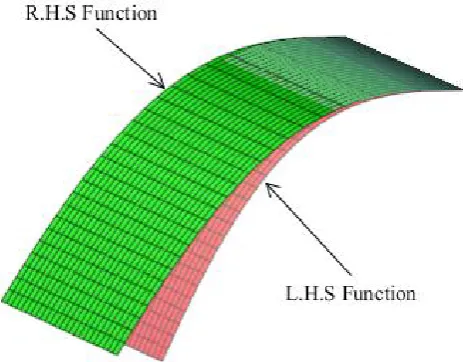
for all x, y ∈ X. Then (X, σ) is a 0-σ-complete metric-like space which is not σ-complete ([11, Example 5]). Let T : X → X be mapping given by Tx = x4. Take F(α) = ln(α) +α and τ = ln 4, where α >0. Then for x > y,
σ(Tx,Ty) = σ
x 4, y 4 = x 4 >0 and
max
σ(x, y), σ(x,x
4), σ(y,
y
4),
σ(x,y4) +σ(y,x4)
4 ,
σ(x,x4), σ(y,y4) 1 +σ(x, y)
= max
x, x, y,x+ max{y, x 4}
4 ,
xy
1 +x
=x.
Hence,
τ+F(σ(Tx,Ty)) = ln 4 + x 4 + ln(
x
4)≤x+ lnx
=F
max
(
σ(x, y), σ(x,Tx), σ(y,Ty),σ(x,Ty)+4σ(y,Tx), σ(x,Tx)σ(y,Ty)
1+σ(x,y)
)
.
Similarly, for x=y6= 0 ( otherwise σ(Tx,Ty) = 0 ) one gets that
τ+F(σ(Tx,Ty)) = ln 4 + x 2 + ln(
x
2)≤2x+ ln 2x
=F
max
(
σ(x, y), σ(x,Tx), σ(y,Ty),σ(x,Ty)+4σ(y,Tx), σ(x,Tx)σ(y,Ty)
1+σ(x,y)
)
.
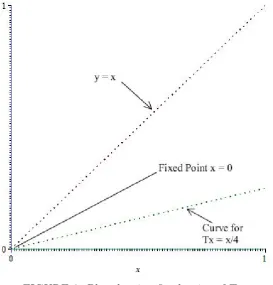
Following figures (Figs. 1,2) show that R.H.S. expression dominates the L.H.S expression in [0,1]∩Q, which validates our inequalities in the example 2.3.
FIGURE 1. Plot of Inequality, 2D view
FIGURE 3. Plot showing fixed point of T
Now, we introduce the notion of F-Suzuki contraction in metric like space and prove a corre-sponding fixed point theorem.
Definition 2.4. Let (X, σ) be a metric like space. A mapping T :X →X is said to be aF-Suzuki contraction if there existsτ > 0 such that for allx, y ∈X with T x6=T y
1
2σ(x, T x)< σ(x, y)⇐⇒τ +F(σ(T x, T y))≤F(σ((x, y)) (2.15)
where F ∈F.
Theorem 2.5. Let (X, σ) be a 0−σ complete metric like space and T : X → X be a F-Suzuki contraction. Then T has a unique fixed point in X.
Proof . Choose x0 ∈X and define a sequence {xn}∞n=1 by
x1 =T x0, x2 =T x1 =T2x0, . . . , xn+1 =T xn=Tn+1x0, ∀ n∈N (2.16)
If there exists n∈N such that σ(xn, T xn) = 0,the proof is complete.
So, we assume that 0< σ(xn, T xn) =σ(xn, xn+1) =σn, ∀ n ∈N.
Therefore
1
2σ(xn, T xn)< σ(xn, T xn), ∀n ∈N (2.17) which implies that
i.e.
F(σ(T xn, T2xn))≤F(σ(xn, T xn))−τ.
Continuing this process, we get
F(σ(xn, T xn)) ≤ F(σ(xn−1, T xn−1))−τ ≤ F(σ(xn−2, T xn−2))−2τ
.. .
≤ F(σ(x0, T x0))−nτ. (2.18)
From (2.18), we get σn=F(σ(xn, T xn))→ −∞as limit n→ ∞.
Thus, from (F2), we have lim
n→∞σn= limn→∞σ(xn, T xn) = 0
Now, by property (F3) there exists k ∈(0,1) such that
lim
n→∞(σn) kF(σ
n) = 0. (2.19)
By (2.19), the following holds for alln ∈N:
(σn)kF(σn)−(σn)kF(σ0)≤(σn)k(−nτ)≤0 (2.20)
passing to limit asn → ∞ in (2.19), using (2.18) and (2.17), we obtain
lim
n→∞n(σn)
k = 0 (2.21)
From, (2.21) there exists n1 ∈N such that n(σn)k ≤1 for all n≥n1.So, we have, for all n ≥n1
σn≤
1
n1/k. (2.22)
Now, using property (σ3) and (2.22), we have for m > n≥n1
σ(xn, xm)≤σ(xn, xn+1) +σ(xn+1, xn+2) +. . .+σ(xm−1, xm)
=%n+%n+1+. . .+%m−1
= Σmi=−1n %i ≤Σi∞=n%i ≤Σ∞i=n
1
n1k
.
By the convergence of the series Σ∞n=1 1
n1k
, passing to limit n→ ∞, we get σ(xn, xm)→0 and hence {xn}is a 0-Cauchy sequence in (X, σ). SinceX is 0-complete metric-like space, there exists a u∈ X
such that limn→+∞xn→u; equivalently,
lim
n,m→∞σ(xn, xm) = limn→∞σ(xn, u) = σ(u, u) = 0. (2.23)
Now, we claim that there exists a subsequence {xnk} of {xn} such that
1
2σ(xnk, T xn)< σ(xnk, u) or 1
2σ(T xnk, T
2x
nk)< σ(T xnk, u), ∀k ∈N. (2.24)
Suppose contrary that there existsk ∈N such that
1
2σ(xnk, T xnk)≥σ(xnk, u) and 1
2σ(T xnk, T
2x
Therefore,
2σ(xnk, u)≤σ(xnk, T xnk)≤σ(xnk, u) +σ(u, T xnk)
which implies that
σ(xnk, u)≤σ(u, T xnk). (2.26)
It follows from (2.24) and (2.26) that
σ(xnk, u)≤σ(u, T xnk)≤ 1
2σ(T xnk, T
2x nk)
Since 12σ(xnk, T xnk)< σ(xnk, T xnk), then by 2.15, we have
τ+F(σ(T xnk, T
2(x
nk)))≤F(σ(xnk, T xnk)). Since τ >0,this imply that
F(σ(T xnk, T
2x
nk))< F(σ(xnk, T xnk)). So, from (F1), we get
σ(T xnk, T
2
xnk)< σ(xnk, T xnk) (2.27)
It follows from (2.24), (2.26) and (2.27) that
σ(T xnk, T
2x
nk)< σ(xnk, T xnk)≤σ(xnk, u) +σ(u, T xnk)
≤ 1
2σ(T xnk, T
2x nk) +
1
2σ(T xnk, T
2x nk)
=σ(T xnk, T
2x nk).
This is a contradiction. Hence (2.24) holds for every k ∈ N, i.e. either τ +F(σ(T xnk, T u)) ≤
F(σ(xnk, u)) is true for every k ∈ N or τ +F(σ(T
2x
nk, T u)) ≤ F(σ(T xnk, u)) = F(σ(xnk+1, u)) is true for every k ∈N.
In first case from (2.23) and (F2), we obtain
lim
n→∞σ(T xnk, T u) = 0.
Therefored(u, T u) = lim
n→∞σ(xnk+1, T u) = limn→∞σ(T xnk, T u) = 0.
Also in the second case using (2.23) and (F2), we get
lim
n→∞σ(T 2
xnk, T u) = 0.
Therefore,d(u, T u) = lim
n→∞σ(xnk+2, T u) = limn→∞σ(T 2x
nk, T u) = 0.
Hence u is a fixed point ofT. The uniqueness of fixed point follows from (2.15).
From (F1) and (2.15), we get the following corollary:
Corollary 2.6. Let (X, σ) be a 0−σ complete metric like space andT :X →X be a mapping such that
1
2σ(x, T x)< σ(x, y)⇐⇒σ(T x, T y))< σ(x, y) (2.28) Then T has a unique fixed point in X.
Example 2.7. Let X and σ be as in Example (2.3). Define T :X →X as follows:
T(x) =
(
1
2, if x= 1,
0, otherwise.
3. An application to second order differential equations
Consider the boundary value problem for second order differential equation of the form
(
x00(t) = −f(t, x(t)), t∈I
x(0) =x(1) = 0. (3.1)
where I = [0,1],f ∈C(I×R,R).
In this section we are going to apply Theorem 2.2 to the study of existence and uniqueness of solutions for a type of second order differential equations. Our approach is inspired by Section 5 of [2].
It is known, and easy to check, that the problem (3.1) is equivalent to the integral equation
x(t) =
Z 1
0
G(t, s)f(s, x(s))ds, for t∈I, (3.2)
where Gis the Green function defined by
G(t, s) =
(
(1−t)s if 0≤s≤t ≤1,
(1−s)t if 0≤t≤s ≤1.
That is, if x ∈ C2(I,R), then x is a solution of problem (3.1) if and only if it is a solution of the integral equation (3.2).
LetX =C(I) be the space of all continuous functions defined onI and kuk∞= maxt∈I|u(t)|for
eachu∈ X. Consider the metric-like σ onX given by
σ(x, y) =kx−yk∞+kxk∞+kyk∞ for all x, y ∈X.
Note thatσ is also a partial metric on X and that
dσ(x, y) := 2σ(x, y)−σ(x, x)−σ(y, y) = 2kx−yk∞.
Hence, (X, σ) is complete as the metric space (X,k · k∞) is complete.
Theorem 3.1. Assume the following conditions:
1. there exist continuous functions α:I →R+ and β :I →
R+ such that
|f(s, a)−f(s, b)| ≤8α(s)|a−b|, for s∈I and a, b∈R,
|f(s, a)| ≤8β(s)|a|, for s ∈I and a∈R;
2. maxs∈Iα(s) = λ1 < 13 and maxs∈Iβ(s) = λ2 < 13.
Then the problem (3.1) has a unique solution u∈ X =C(I,R).
Proof . Define the self-mapT :X → X by
Tx(t) =
Z 1
0
for allx ∈ X and t∈I. Then, the problem (3.1) is equivalent to finding a fixed point u of T in X. Letx, y ∈ X. We have
|Tx(t)− Ty(t)|=
Z 1 0
G(t, s)f(s, x(s))ds−
Z 1
0
G(t, s)f(s, y(s))ds
≤ Z 1 0
G(t, s)|f(s, x(s))−f(s, y(s))|ds
≤8
Z 1
0
G(t, s)α(s)|x(s)−y(s)|ds
≤8λ1kx−yk∞sup t∈I
Z 1
0
G(t, s)ds
=λ1kx−yk∞.
Next, we recall that for each t∈I one hasR01G(t, s)ds = t(1−2t), and then
sup
t∈I
Z 1
0
G(t, s)ds= 1 8.
Therefore,
kTx− Tyk∞ ≤λ1kx−yk∞. (3.3)
Moreover, we have
|Tx(t)|=
Z 1 0
G(t, s)f(s, x(s))ds
≤ Z 1 0
G(t, s)|f(s, x(s))|ds
≤8
Z 1
0
G(t, s)β(s)|x(s)|ds ≤8λ2kxk∞sup t∈I
Z 1
0
G(t, s)ds
≤λ2kxk∞.
Thus
kTxk∞ ≤λ2kxk∞, (3.4)
and also
kTyk∞ ≤λ2kyk∞. (3.5)
Assuminge−τ =λ1+ 2λ2 <1 (τ ∈R+). Using (3.3)–(3.5), we obtain
σ(Tx,Ty) =kTx− Tyk∞+kTxk∞+kTyk∞ ≤λ1kx−yk∞+λ2kxk∞+λ2kyk∞
≤(λ1+ 2λ2)(kx−yk∞+kxk∞+kyk∞)
=e−τσ(x, y)≤e−τ
max
σ(x, y), σ(x,Tx), σ(y,Ty),σ(x,Ty) +σ(y,Tx)
4 ,
σ(x,Tx)σ(y,Ty) 1 +σ(x, y) .
Taking the functionF :R+ →
R defined by F(α) = lnα, belonging to F we get
τ +F(σ(Tx,Ty))≤F
max
σ(x, y), σ(x,Tx), σ(y,Ty),σ(x,Ty) +σ(y,Tx)
4 ,
σ(x,Tx)σ(y,Ty) 1 +σ(x, y) .
4. An application to fractional differential equations
In this section, we apply Theorem 2.2 to establish the existence of solution of fractional order func-tional differential equation.
Consider the following initial value problem (IVP for short) of the form
Dαy(t) = f(t, yt), for each t∈J = [0, b],0< α <1, (4.1)
y(t) =φ(t), t∈(−∞,0] (4.2)
where Dα is the standard Riemann-Liouville fractional derivative, f : J×B →
R, φ ∈ B, φ(0) = 0
and B is called a phase space or state space satisfying some fundamental axioms (H-1, H-2, H-3) given below which were introduced by Hale and Kato in [5].
For any functiony defined on (−∞, b] and any t ∈J , we denote byyt the element of B defined by
yt(θ) = y(t+θ), θ ∈(−∞,0].
Here yt(·) represents the history of the state from −∞up to present time t.
ByC(J,R) we denote the Banach space of all continuous functions from J intoR with the norm
||y||∞:= sup{|y(t)|:t ∈J}
where | · |denotes a suitable complete norm on R.
Now consider the metric like space σ onX given by
σ(x, y) = 2d(x, y) for all x, y ∈X.
Then, (X, σ) is complete as the metric space (X, d) is complete.
(H-1) If y: (−∞, b]→R, and y0 ∈B, then for every t∈[0, b] the following conditions hold:
(i) yt is in B,
(ii) ||yt||B ≤K(t) sup{|y(s)|: 0≤s≤t}+M(t)||y0||B,
(iii) |y(t)| ≤H||yt||B,
where H ≥ 0 is a constant, K : [0, b] → [0,∞) is continuous, M : [0,∞) → [0,∞) is locally bounded and H, K, M are independent of y(·).
(H-2) For the function y(·) in (H-1), yt is a B-valued continuous function on [0, b].
(H-3) The space B is complete.
By a solution of problem (4.1)-(4.2), we mean a space Ω = {y : (−∞, b] → R : y|(−∞,0] ∈
B and y|[0,b] is continuous}. Thus a function y ∈ Ω is said to be a solution of (1)-(2) if y satisfies
the equation Dαy(t) = f(t, yt) on J, and the condition y(t) =φ(t) on (−∞,0].
The following lemma is crucial to prove our existence theorem for the problem (4.1)-(4.2).
Lemma 4.1. (See [4].) Let 0< α <1 and let h: (0, b]→R be continuous and lim
t→0+h(t) =h(0 +)∈
R. Theny is a solution of the fractional integral equation
y(t) = 1 Γ(α)
Z t
0
if and only if y is a solution of the initial value problem for the fractional differential equation
Dαy(t) =h(t), t ∈(0, b],
y(0) = 0.
Now we are ready to prove following existence theorem.
Theorem 4.2. Let f :J×B →R. Assume (H) there exists q >0 such that
|f(t, u)−f(t, v)| ≤q||u−v||B, for t ∈J and every u, v ∈B.
If bαKbq
Γ(α+1) =λ <1 where
Kb = sup{|K(t)|:t∈[0, b]},
then there exists a unique solution for the IVP (4.1)-(4.2) on the interval (−∞, b].
Proof . To prove the existence of solution for the IVP (4.1)-(4.2), we transform it into a fixed point problem. For this, consider the operator N : Ω→Ω defined by
N(y)(t) =
(
φ(t) t∈(−∞,0],
1 Γ(α)
Rt
0(t−s)
α−1f(s, y
s)ds t ∈[0, b].
Letx(·) : (−∞, b]→Rbe the function defined by
x(t) =
φ(t) t∈(−∞,0],
0 t ∈[0, b].
Then x0 =φ. For eachz ∈C([0, b],R) withz(0) = 0, we denote by ¯z the function defined by
¯
z(t) =
0 if t∈(−∞,0], z(t) if t∈[0, b].
Ify(·) satisfies the integral equation
y(t) = 1 Γ(α)
Z t
0
(t−s)α−1f(s, ys)ds,
we can decomposey(·) asy(t) = ¯z(t) +x(t),0≤t≤b, which impliesyt = ¯zt+xt,for every 0 ≤t≤b,
and the function z(·) satisfies
z(t) = 1 Γ(α)
Z t
0
(t−s)α−1f(s,z¯s+xs)ds
Set
C0 ={z ∈C([0, b],R) :z0 = 0},
and let|| · ||b be the seminorm in C0 defined by
C0 is a Banach space with norm || · ||b. Let the operator P :C0 →C0 be defined by
(P z)(t) = 1 Γ(α)
Z t
0
(t−s)α−1f(s,z¯s+xs)ds, t∈[0, b]. (4.3)
That the operatorN has a fixed point is equivalent to P has a fixed point, and so we turn to proving that P has a fixed point. Indeed, consider z, z∗ ∈C0. Then we have for each t ∈[0, b]
|P(z)(t)−P(z∗)(t)| ≤ 1
Γ(α)
Z t
0
(t−s)α−1|f(s,z¯s+xs)−f(s,z¯s∗+xs)| ds
≤ 1
Γ(α)
Z t
0
(t−s)α−1q||z¯s−z¯∗s||B ds
≤ 1
Γ(α)
Z t
0
(t−s)α−1qKb sup s∈[o,t]
||z(s)−z∗(s)|| ds
≤ Kb
Γ(α)
Z t
0
(t−s)α−1q ds ||z−z∗||b.
Therefore
||P(z)−P(z∗)||b ≤
qbαK b
Γ(α+ 1)||z−z
∗|| b,
i.e.
σ(P(z), P(z∗))≤λσ(z, z∗).
By passing through logarithm, we write lnσ(P(z), P(z∗))≤ln(e−τσ(z, z∗)) (where λ=e−τ >0) and hence
τ +F((σ(P(z), P(z∗)))≤F((σ(z, z∗))
≤F
max
(
σ(z, z∗), σ(z, P(z)), σ(z∗, P(z∗)),σ(z,P(z∗)+4σ(z∗,P(z)), σ(z,P(z))σ(z∗,P(z∗))
1+σ(z,z∗)
)
.
Now we observe that the function F :R+ →
Rdefined by F(u) = lnu for each u∈R+, then F ∈ F
and so we deduce that the operatorP satisfies all the hypothesis of Theorem 2.2. ThusP has unique fixed point.
5. Conclusion
Taking into account its interesting applications, searching for fixed point theorems involving new contractive type conditions in abstract spaces has received considerable attention through the last few decades. In this connection, the main aim of our paper is to present new concepts of rational
´
Ciri´c type generalizedF-contraction and F-Suzuki contraction in a metric-like space and utilize the same to establish fixed point results. Two applications to initial and boundary value problems are illustrated to the usability of the obtained fixed point results.
Acknowledgements
(No. 2052/FNPDR/2015). The fourth author gratefully acknowledges with thanks the Department of Research Affairs at UAEU. This article is supported by the grant: UPAR (11) 2020, Fund No. 31S249 (COS).
References
[1] A. Amini Harandi, Metric-like spaces, partial metric spaces and fixed points, Fixed Point Theory Appl., 2012 (2012): 204.
[2] H. Aydi and E. Karapinar,Fixed point results for generalizedα−ψ-contractions in metric-like spaces and appli-cations, Electronic J. Diff. Eq., 133 (2015) 1–15.
[3] M. Bukatin, R. Kopperman, S. Matthews and H. Pajoohesh, Partial metric spaces, Amer. Math. Monthly, 116 (2009) 708–718.
[4] D. Delboso and L. Rodino, Existence and uniqueness for a nonlinear fractional differential equation, J. Math. Anal. Appl., 204 (1996) 609–625.
[5] J. Hale and J. Kato, Phase space for retarded equations with infinite delay, Funkcial. Ekvac. 21 (1978)11-41. [6] E. Karapinar and P. Salimi,Dislocated metric space to metric spaces with some fixed point theorems,Fixed Point
Theory Appl., 2013 (2013): 222.
[7] S. G. Matthews, Partial metric topology, Proc. 8th Summer Conference on General Topology and Applications, Ann. New York Acad. Sci., 728 (1994) 183–197.
[8] G. Minak, A. Helvacı and I. Altun, Ciri´´ c type generalized F-contractions on complete metric spaces and fixed point results, Filomat, 28 (2014) 1143–1151.
[9] H. Piri and P. Kumam, Some fixed point theorems concerning F-contraction in complete metric spaces, Fixed Point Theory Appl., 2014 (2014): 210.
[10] N. Shobkolaei, S. Sedghi, J. R. Roshan and N. Hussain,Suzuki type fixed point results in metric-like spaces, J. Function Spaces Appl. (2013) Article ID 143686,9 pages.
[11] S. Shukla, S. Radenovi´c and V. ´Cojbaˇsi´c Raji´c, Some common fixed point theorems in 0-σ-complete metric-like spaces, Vietnam J. Math., 41 (2013) 341–352.
[12] S. Shukla and S. Radenovi´c, Some common fixed point theorems for F-contraction type mappings in 0-complete partial metric spaces, J. Math. (2013) 2013, Article ID 878730, 7 pageS.
[13] S. Shukla, S. Radenovi´c and Z. Kadelburg, Some fixed point theorems for ordered f-generalized contractions in 0-f-orbitally complete partial metric spaces, Theory Appl. Math. Comput. Sci., 4 (2014) 87–98.
[14] D. Wardowski,Fixed points of a new type of contractive mappings in complete metric spaces, Fixed Point Theory Appl., 2012 (2012): 94.