A hybrid method combining the FDTD and a time domain
boundary-integral equation marching-on-in-time algorithm
A. Becker and V. Hansen
Lehrstuhl f¨ur Theoretische Elektrotechnik der Universit¨at Wuppertal, Rainer-Gruenter-Str. 21, 42119 Wuppertal, Germany
Abstract. In this paper a hybrid method combining the FDTD/FIT with a Time Domain Boundary-Integral Marching-on-in-Time Algorithm (TD-BIM) is presented. In-homogeneous regions are modelled with the FIT-method, an alternative formulation of the FDTD. Homogeneous regions (which is in the presented numerical example the open space) are modelled using a TD-BIM with equivalent electric and magnetic currents flowing on the boundary between the in-homogeneous and the in-homogeneous regions. The regions are coupled by the tangential magnetic fields just outside the in-homogeneous regions. These fields are calculated by making use of a Mixed Potential Integral Formulation for the netic field. The latter consists of equivalent electric and mag-netic currents on the boundary plane between the homoge-neous and the inhomogehomoge-neous region. The magnetic currents result directly from the electric fields of the Yee lattice. Elec-tric currents in the same plane are calculated by making use of the TD-BIM and using the electric field of the Yee lattice as boundary condition. The presented hybrid method only needs the interpolations inherent in FIT and no additional in-terpolation. A numerical result is compared to a calculation that models both regions with FDTD.
1 Introduction
The FDTD-Method is a very efficient and accurate technique for solving bounded electromagnetic field problems. For the analysis e.g. of scattering or antenna problems including the open space the solution space must be kept finite by intro-ducing an absorbing boundary condition (ABC). An often applied ABC is obtained by introducing a perfectly matched layer (PML), the effect of which is incorporated into the solution-procedure by regarding the PML-region as a part of the FDTD solution space, that means, by treating it within the FDTD scheme. As the FDTD is a “local” method the PML
Correspondence to: A. Becker
can be regarded as a “local” ABC, too. A “global” ABC is obtained if an integral formulation for a surface inclosing the bounded FDTD solution space is used as a starting point. As an example for such a “global” FDTD-ABC formulation (de Moerlosse et al., 1993) shall be mentioned, where the magnetic field is calculated just outside the FDTD solution space by an integral equation. As the Yee-scheme consist-ing of two shifted lattices does not provide the required elec-tric and magnetic currents in the same plane, one of these must be calculated by an additional interpolation. A very in-teresting class of TD-integral formulations are the so called Time Domain Boundary-Integral Marching-on-in-Time Al-gorithms (TD-BIMs), which in the last few years draw more an more attention. By this, the two main drawbacks of TD-BIMs -stability problems and high computational cost- have been more and more alleviated (e.g. Shanker et al., 2000). Thus, it is reasonable to make use of these advantages and to develop a hybrid method that combines the FDTD/FIT and a TD-BIM, in other words, to make use of the TD-BIM as a “global” ABC for the FDTD solution space.
This paper is organized as follows:
– Section 2 gives an overview of the TD-BIM that is used here to calculate the electric current density at the boundary between the inhomogeneous and the homoge-neous body.
– Section 3 shortly repeats the differences between the FDTD and the FIT. The latter is used here to model in-homogeneous bodies.
– Section 4 explains the algorithm of the hybrid method proposed here which combines both numerical tech-niques.
– Section 5 shows a first numerical example to test the method.
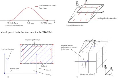
Fig. 1. Temporal and spatial basis function used for the TD-BIM.
Fig. 2. Spatial allocation of the electric and the magnetic grid voltages and the straightforward allocation of the magnetic current.
2 TD-BIM
The time domain electric field integral equation (TD-EFIE) for a homogeneous infinite space is given to:
E(r, t )= −∂A(r, t )
∂t − ∇φ (r, t )− 1
ε∇ ×F(r, t ) . (1) When applying the equivalence principle the potentials are related to the equivalent surface sources of the field by
A(r, t )= µ 4π
Z
A0
J(r0, t−R c)
R da
0
, (2)
φ (r, t )= 1 4π ε
Z
A0
ρ(r0, t−R c)
R da
0
, (3)
F(r, t )= ε 4π
Z
A0
M(r0, t−R c)
R da
0 (4)
withR =r−r0
and the region outside ofA0source free.
The surface A0 is the surface on which the currents flow, the so called Huygens-surface. The substitution of Eq. (2), Eq. (3) (together with the continuity equation∇J+∂
∂tρ=0)
and Eq. (4) into Eq. (1) results into a relationship between the electric field and the electric and the magnetic current densi-ties (Rao, 1999):
E(r, t )= Z
A0
"
− µ
4π ∂ ∂t
J(r0, t−R c)
R
+∇ Rt−Rc
0 ∇J r
0, t
dt
4π εR − ∇ ×
M(r0, t−R c)
4π R
#
da0. (5)
For the numerical solution the surfaceA0is subdivided into small patches. The electric and magnetic current density is numerically approximated as a series of unknown coef-ficients multiplied with basis functions:
J(r, t )= Ns X
i=0
Nt X
j=0
J(i,j )βi(r) τj(t ) ,
M(r, t )= Ns X
i=0
Nt X
j=0
M(i,j )βi(r) τj(t ) (6)
Ns andNt are the numbers of space samples and the time
step in which the electric field is calculated, respectively. The spatial and temporal basis functions applied here are shown in Fig. 1. The width of the temporal basis function is 24TBEM. We integrate the combination of Eqs. (5) and
(6) multiplied with a test functionβkover the domainAk of
the test function (Sarkar et al., 2000):
Z
Ak
E(r, t )βk(r)da= Z
Ak Z
A0
Ns X
i=0
Nt X
j=0
"
− µ
4π
J(i,j )βk(r)βi r0τ0 t−Rc
R
− Rt−Rc
0 J(i,j )γk(r)γi r 0
τ (t ) dt 4π εR
−∇ ×M(i,j )βk(r)βi r 0
τ t−R c
4π R
#
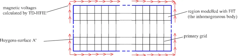
Fig. 3. The allocation of the Huygens-surfaceA0in the Yee lattice.
The term γ represents the surface-divergence of the basis functionβ. Equation (7) connects the tangential electric field on surfaceAk to the electric and the magnetic currents
flow-ing on surfaceA0. The equivalence principle relates the tan-gential electric field on the surfaceAkto the equivalent
mag-netic current:
βk·(n×M)=βk·(n×(E×n))
=βk·[E(n·n)−n·(n·E)]=βk·E (8)
Substituting Eq. (8) into Eq. (7) leads to a relationship be-tween the electric and magnetic current density:
Z
Ak N X
i=1
M(i,Nt)βk·(n×βi(r)) da=
Z Ak Z A0 N X
i=1
Nt X
j=1
"
− µ
4π
J(i,j )βk(r)βi r0
τ0 t−R c
R
− Rt−Rc
0 J(i,j )γk(r)γi r0
τ (t ) dt 4π εR
−∇ ×M(i,j )βk(r)βi r 0
τ t−R c
4π R
#
da0da. (9) If the actual magnetic current density on surfaceA0is known, the actual electric current density can be calculated from the electric current density retarded in time at least one time step and from the magnetic current density by enforcing continu-ity on all subdomainsAkofA0. Eq. (9) can be written as:
Z1,1 . . . Z1,N
..
. . .. ... ZN,1. . . ZN,N
| {z }
Z
I1,Nt
.. . IN,Nt
=f N X
i=1
Nt−1 X
j=1 J(i,j )
!
+g
N X
i=1
Nt X
j=1 M(i,j )
! = PN i=1
PNt−1
j=1 Y(1,i,j )J(i,j )+PNi=1
PNt
j=1X(1,i,j )M(i,j )
.. .
PN i=1
PNt−1
j=1 Y(N,i,j )J(i,j )+PNi=1
PNt
j=1X(N,i,j )M(i,j )
(10) The matrix Z describes the actual electric fields produced by the actual electric currents and thus is highly sparse. In a
time-invariant system bothZand the coefficientsX(k,i,j )and
Y(k,i,j ) have to be calculated just once, at the first time step.
If the tangential electric field equals zero (that means the ma-terial is a perfect electric conductor and there is no magnetic current density) Eq. (10) will be sufficient for calculating the electric current density in a marching-on-in-time algorithm (MoT). Otherwise a second equation is needed to calculate both current densities. In our case we will use the FIT to up-date the magnetic current density and Eq. (10) to upup-date the electric current density. Thus the surfaceA0will encase the region modelled with FIT.
3 FDTD/FIT
The TD-FIT can be considered as a special formulation of the FDTD-method (Weiland, 1996). In contrast to FDTD it is based on the Maxwell Equations in integral form. By using electric and magnetic fluxes and grid voltages as un-known coefficients and by using the Yee lattice to allocate them, these equations can be written as:
Ceˆ= −∂ ∂t
ˆˆ
b (11)
e
Chˆ = ∂ ∂t
ˆˆ
d+jˆˆ. (12)
ˆ
erepresents the grid voltage above one LineLi of the Yee
cell. The termdˆˆrepresents the flux through one AreaAi of
the Yee cell. The unknown coefficients can be considered as the analytic – and thus numerically error-free – values. The application of Eq. (12) is illustrated in Fig. 2a. A second order accurate central difference approximation for the time derivative leads to the leap frog algorithm. The definition of grid voltages as unknown coefficients is essential if using the FIT instead of FDTD for our hybrid method.
4 Hybrid method
Fig. 5. The boundary of the FIT-domain and the resulting minimal retardation in the calculation of the magnetic grid voltages.
4.1 Basic features
We interconnect the inhomogeneous body and the surround-ing homogeneous region by calculatsurround-ing tangential magnetic grid voltages just outside the inhomogeneous body using a TD magnetic field integral equation (TD-HFIE) which uses electric and magnetic currents flowing on the Huygens-surfaceA0whose location is shown in Fig. 3.
The magnetic current on the surface A0 results directly from the electric grid voltages of the FIT, which will be shown beneath. Due to the fact that the magnetic grid volt-ages are spatially (and temporally) separated from the elec-tric grid voltages the elecelec-tric currents on the Huygens-surface A0 can not be calculated from the magnetic grid voltages. Therefore the electric current will be calculated by using a TD-BIM -as described in Sect. 2 – which is capable of con-sidering bodies outside the FIT volume.
To develop the algorithm of the hybrid method we start with the FIT and a Cartesian grid. The unknowns in FIT are grid voltages defined as:
ˆ ei =
Z
Li
Eds,hˆi = Z
Li
Hds (13)
As already mentioned we use the rooftop basis function for the TD-BIM because the discretization for FIT leads to a patch model of the surfaceA0 consisting of rectangular el-ements (see Fig. 2) if Cartesian Coordinates are used. The unknowns in the TD-BIM are proportional to the flux orthog-onal to these edges. With the location in time of the magnetic current density according to Fig. 4 this results into the fol-lowing relationship between the unknowneˆi of the FIT and
the magnetic current of the TD-BIM (see Fig. 2b):
Z
Li
MNte3=
Z
Li
e2×ENte3ds=
Z
Li
ENte1ds= ˆei,Nt (14)
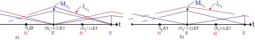
Now the magnetic current density can be calculated from the electric grid voltages by using Eq. (14). The electric currents are located at the same time step like the magnetic currents (see Fig. 4a). It is possible to locate the electric currents at the same time step like the magnetic grid voltages and even to use a time step4TBEM for the electric currents which is
larger than the time step given by FIT (see Fig. 4b). The latter decreases calculation time and improves stability because the time step given by the FIT is extremely small.
4.2 Time stept =Nt4T
The calculation of the magnetic grid voltages interconnecting the inhomogeneous and the homogeneous region (see Fig. 3) with the TD-HFIE is equivalent to the use of the so called pulse-test-function:
Z
S
Hds= Z
A
H βpulseda, with βpulse =
ds
|ds| rS
(15) The electric and magnetic current density is approximated according to Sect. 2. Thus the magnetic grid voltages can be calculated by combining Eq. (7) and the Fitzgerald-transformation/duality. The use of a pulse-test-function al-lows us to calculate the magnetic grid voltages without the need to calculate a term proportional to 1/r2. As seen in Fig. 5a the minimum distance between boundary plane and magnetic grid voltages is 0.5Lminwhich is half of the
small-est spatial discretization. In Fig. 5a the distance between the Huygens-surface and the magnetic grid voltages is half a cell-size.
In our numerical example we will use one and a half cell-sizes between Huygens-surface and the grid voltages calcu-lated by the TD-HFIE (see Fig. 6a). Due to the Courant con-dition the minimal temporal retardation can be calculated to:
τmin =
Lmin
c = √
3c4T c =
√
Fig. 6. Geometry and electric fields at the boundary of the FIT-volume.
Fig. 7. The electric fields at the boundary of the FIT-volume.
As seen in Fig. 5b the actual magnetic grid voltages are not functions of the actual electric and magnetic currents. Thus the grid voltages can be calculated by using expired currents only.
4.3 Time stept =(Nt+0.5)4T
If the tangential magnetic grid voltages are known the FIT-algorithm can be completed in the interior and on the bound-ary as usual (t = (Nt +0.5)4T). Consequently, the
elec-tric grid voltages are known in the whole interior and on the boundary. With Eq. (14) the magnetic currents can be calcu-lated in a very efficient way. Anyway, the FIT does not give a relationship between the magnetic and the electric fields in one common plane. At the next time-step (t=(Nt+1)4T)
the magnetic as well as the electric currents at time steps t =(Nt +0.5)4T are needed. The latter are calculated by
applying Eq. (10) att=(Nt+0.5)4T. As boundary
condi-tion we use the electric fields calculated by FIT (proporcondi-tional to the magnetic flux as related by Eq. 14), i.e. the fields cal-culated by the TD-IE must equal the fields calcal-culated by the FIT. Now both electric and magnetic currents are known on the surfaceA0.
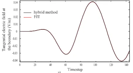
5 Numerical results
As a first numerical evaluation of the hybrid method we sim-ulate an electric source (sinusoidal, 500 MHz) in the interior of an air filled cube (see Fig. 6a) by impressing one electric grid voltage. This source reflects all incoming waves and so it acts like a small wire. The spatial and temporal dis-cretization is determined by the Courant condition, assuming a 1.1 GHz source and 20 cells per wavelength. The cube is 6×7×8-cells big. Between the Huygens-surface and the FIT-boundary we put one layer. As an example we calculate one electric grid voltage on the Huygens-surface. The re-sult is compared to a calculation in which a cube with PMC-boundary condition is simulated. This simulation contains so many cells in each direction that waves at the boundary can be neglected. The results agree well despite of the extremely small distance between boundary and source. However, af-ter approximately 12 periods the calculation with the hybrid method becomes unstable. Such instabilities are typical for TD-BIMs and the accuracy and stability strongly depends on the numerical evaluation of the matrix Z and the coefficients X(k,i,j )andY(k,i,j ). So it can expected be that these
implemented numerical integration. The efficiency can be drastically increased by using techniques like the plane wave time domain algorithm (Shanker, 2000).
IEEE Trans. AP, 48, 1625–1634, 2000.
Shanker, B., Ergin, A., Ayg¨u, K., and Michielssen, E.: Analysis of Transient Electromagnetic Scattering Phenomena Using a Two-Level Plane Wave Time-Domain Algorithm, IEEE Trans. AP, 48, 510–523, 2000.