O. Lange1and B. Yang2
1Robert Bosch GmbH, Robert-Bosch-Strasse 200, 31139 Hildesheim, Germany
2Chair of System Theory and Signal Processing, Universit¨at Stuttgart, Pfaffenwaldring 47, 70569 Stuttgart, Germany
Abstract. This paper focuses on the estimation of the direction-of-arrival (DOA) of signals impinging on a sensor array. A novel method of array geometry optimization is pre-sented that improves the DOA estimation performance com-pared to the standard uniform linear array (ULA) with half wavelength element spacing. Typically, array optimization only affects the beam pattern of a specific steering direction. In this work, the proposed objective function incorporates, on the one hand, a priori knowledge about the signal’s DOA in terms of a probability density function. By this means, the ar-ray can be adjusted to external conditions. On the other hand, a modified beam pattern expression that is valid for all possi-ble signal directions is taken into account. By controlling the side lobe level and the beam width of this new function, DOA ambiguities, which lead to large DOA estimation errors, can be avoided. In addition, the DOA fine error variance is min-imized. Using a globally convergent evolution strategy, the geometry optimization provides array geometries that signif-icantly outperform the standard ULA with respect to DOA estimation performance. To show the quality of the algo-rithm, four optimum geometries are presented. Their DOA mean squared error is evaluated using the well known de-terministic Maximum Likelihood estimator and compared to the standard ULA and theoretical lower bounds.
1 Introduction
This paper deals with the problem of estimating the direction-of-arrival (DOA) of signals impinging on an array of spatially distributed sensors. There exists a vast amount of DOA estimators, whose performance and accuracy com-pared to theoretical lower bounds like the Cram´er-Rao lower
Correspondence to: O. Lange ([email protected])
bound have been intensively investigated. A good introduc-tion to array signal processing and DOA estimaintroduc-tion can be found in (Krim and Viberg, 1996) and the references therein. In this work, we focus on the deterministic Maximum Like-lihood (DML) DOA estimator, which is asymptotically sistent and statistically efficient under certain regularity con-ditions (Stoica and Nehorai, 1989). Nevertheless, any other estimator that works with an arbitrary array geometry can be applied to the results of this work, as well.
Given a fixed number of sensor elements, the question of an optimum sensor placement with respect to DOA estima-tion performance naturally arises. In this context, it is intu-itively clear that no “globally optimal” geometry for DOA estimation exists. Instead, an array geometry is always opti-mal with respect to certain presuppositions like the number of signals (Gershman and B¨ohme, 1997), the statistical prop-erties of the DOA or the probability of large DOA estimation errors, etc.
Although there exist many different approaches to achiev-ing an optimum geometry, basically all of them can be at-tributed directly or indirectly to the array beam pattern in terms of the side lobe level (SLL) and the shape of the main lobe. Because shape is a quantity that is difficult to charac-terize mathematically, the half power beam width (HPBW) is often used as a feature instead. It corresponds to the ac-curacy of the DOA estimates, i.e. the narrower the main beam, the lower the variance of the DOA estimates. Thus, the main beam width is directly related to the Cram´er-Rao lower bound, which represents the minimum variance of an unbiased estimator (van Trees, 2002). Furthermore, a narrow beam width increases the possibility of angular signal sepa-rability in the multiple signal case.
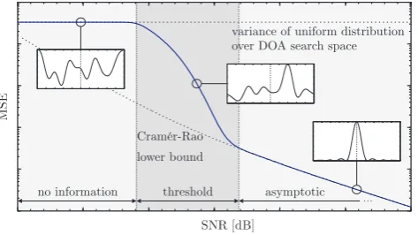
Fig. 1. Typical MSE curve of DOA estimation with three different regions of operation. In addition, likelihood functions are plotted corresponding to the asymptotic, the threshold and the no informa-tion region, respectively.
whose probability of occurrence depends on the SLL of the beam pattern (Athley, 2005).
Moreover, in the multiple signal case, a low SLL prevents high SNR signals from overlapping low SNR signals.
By further reducing the SNR (or the sample size), the MSE goes to saturation, which can be approximated by the vari-ance of a uniform distribution over the DOA search space (Richmond, 2006). Figure 1 quantitatively illustrates this typical DOA MSE curve and presents three regions of op-eration:
1. The asymptotic region is influenced by the shape of the main lobe, i.e. the HPBW; it can be approximated by the Cram¨er-Rao lower bound or the equivalent asymptotic variance of the estimator, respectively.
2. The threshold region is dominated by outliers, whose probability of occurrence is proportional to the SLL. 3. In the no information region, the SNR (or the sample
size) is very low which leads to DOA estimates that are uniformly distributed over the search space.
All attempts of array geometry optimization that aim at DOA performance improvement have to take this MSE character-istic, which is based on a trade-off between SLL and beam width of the beam pattern, into account. In doing so, it should also be noted, that the beam pattern has to be unambigu-ous for all steering directions, where targets are to be ex-pected. Ambiguities and high side lobes in this region should be avoided, as they lead to outliers in DOA estimation, even in high SNR regimes. As the usual beam pattern only rep-resents the array response to a unit wave from a certain di-rection, we introduce a modified beam pattern (MBP), using a simple parameter transformation. By this means, the MBP allows for control of the HPBW and the SLL simultaneously for all valid steering directions.
Fig. 2. Array geometry withNelements on the x-axis with nonuni-form inter element spacings and one far field source at azimuth an-gle2.
To take “real world” external conditions into account, we further incorporate a probability density function (PDF), de-fined for all valid steering directions. It is affected, for in-stance, by the angular a priori distribution of the target’s DOA, the element factor of the sensors, the transmit beam pattern and the effect of blinds or radomes. This a priori PDF is applied as an angular dependent weighting factor to the MBP. By this means, we expand an approach by Oktel and Moses (2005), how previous knowledge about the DOA and hardware characteristics can easily be transferred into the array design process.
Using a globally convergent optimization routine, the HPBW and the SLL of the weighted MBP can now be con-trolled resulting in array geometries that outperform the stan-dard uniform linear array (ULA) with half wavelength ele-ment spacing in terms of DOA estimation accuracy.
This paper is organized as follows. The data model and the MBP are introduced in Sect. 2. We also derive the weighted MBP, which additionally uses a priori knowledge in terms of a beta distributed PDF. Furthermore, we intro-duce the deterministic Maximum Likelihood DOA estimator and show, how prior knowledge can improve DOA estima-tion. In Sect. 3, the objective function for array geometry optimization is defined. Some examples for optimum array geometries are presented and their DOA estimation perfor-mance is compared to the standard ULA using Monte Carlo simulations and the Cram´er-Rao lower bound.
2 Data model and modified beam pattern
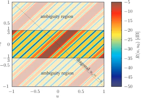
Fig. 3. ULA beam patternR(u,u0)for varying target directions
u0= −1,...,1. For|u0|>13, DOA estimates are ambiguous due to
grating lobes in the beam pattern.
assumed to hold so that the complex baseband array output vector can be modeled by (van Trees, 2002)
x(k)=A(u0)s(k)+n(k), k=1,...,K (1) where A(u0)=
a(u0,1),...,a(u0,Q)
is the (N×Q) ar-ray steering matrix withu0,q=sin20,q,q=1,...,Q. The complex baseband source signals are denoted by s(k)=
s1(k),...,sQ(k)T where(·)T means transpose,n(k)is the additive noise vector based on a Gaussian random process with zero mean and varianceσn2. The number of snapshots is denoted byK. The SNR of theq-th signal at each of the sensors is defined as
SNRq= 1 K
PK
k=1|sq(k)|2 σ2
n
, q=1,...,Q. (2)
The steering matrix A(u0) consists of Q steering vectors a(u0)whosen-th element is defined by
an(u0)=ej
2π
λpx,nu0, n=1,...,N. (3)
Here, the element positions are denoted bypx,nandλis the wavelength.
2.1 Derivation of the modified beam pattern
The normalized array beam patternR(u,u0)is defined as the squared magnitude of the response to a unit wave (s(k)=
1∀k) from directionu0in the case of no noise, i.e. R(u,u0)=
1
NaH(u)a(u0) 2 = 1 N PN n=1e−j
2π
λpx,n(u−u0)
2 , (4)
where the superscript(·)H denotes conjugate transpose. Fig-ure 3 exemplarily shows the beam patterns corresponding to
Fig. 4. Modified beam pattern (MBP) for an ULA with inter ele-ment spacing of34λ.
an 8-element ULA with element spacing 34λ. The steering direction is varied fromu0= −1,...,1. Due to violation of the spatial sampling theorem (van Trees, 2002), the region for unambiguous DOA estimates is limited to|u0|<13 as in-dicated in Fig. 3.
It can be clearly seen from Fig. 3, that knowledge of
r(u)˜ =R(u,u˜ 0= − ˜u)= 1 N N X
n=1
e−j2λπpx,n2u˜ 2 (5)
with−1≤ ˜u≤1, which represents the diagonalu0= −uin Fig. 3, allows for perfect reconstruction of all beam patterns1 R(u,u0)=r(u)˜ |u˜=u−u0
2
. (6)
This means, thatR(u,u0)can be reduced tor(u)˜ without any loss of information. Note that (Eq. 6) is only valid for omni-directional sensor elements. Non uniform element charac-teristics are taken into account in the next subsection where prior knowledge is considered.
The functionr(u)˜ from (Eq. 5) is denoted as the modified beam pattern (MBP), because it can be obtained from the beam pattern by a simple rearrangement of the argumentsu andu0. Figure 4 plots the MBP for the same parameters as in Fig. 3. Note that the region of unambiguous DOA estimates can be identified as−2
3<u˜= u−u0
2 < 2
3 which leads to the prior result|u0|<13 for−1≤u≤1.
2.2 Definition of the a priori PDF
In many array signal processing applications, restrictive as-sumptions can be made concerning the statistical properties of the target’s DOA. Hence, the probability of appearance or detection of a target at a certain directionu0is not uniform for all possible target directions−1≤u≤1. Often, a target is
1To distinguish betweenR(u,u
0)andr(u)˜ , we useu˜instead of
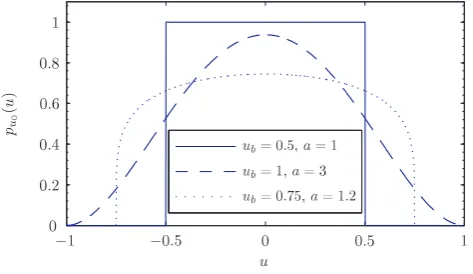
Fig. 5. Different beta probability densities, transformed touspace, from (Eq. 8) withb=afor several values ofubanda.
more likely to appear near the array boresight than laterally. Or there might be a certain region, e.g. in surveillance appli-cations, where the possibility of occurrence of a target is near zero. In addition, incoming signals from certain DOA’s can be damped by the use of hardware constraints like blinds or radomes or by the influence of the array element factor. Fur-thermore, there are applications like automotive radar, where targets are actively illuminated by a transmit antenna. Ne-glecting the influence of multi path scattering, the DOA an-gular distribution directly corresponds to the beam shape of the transmit antenna.
Thus, the mentioned characteristics directly or indirectly affect the statistical properties of the target’s DOA. To ac-count for the mentioned effects, we introduce the the PDF pu0(u)which represents the angular a priori information. In
this work, we focus (without loss of generality) on the beta distribution
p(v)=
1
B(a,b)v
a−1(1−v)b−10≤v≤1
0 elsewise, (7)
whereB(a,b)=R1
0va
−1(1−v)b−1dv is the beta function. The parametersaandbare real positive constants. A trans-formation of the random variablev∈ [0,1]touspace with u∈ [−ub,ub], 0< ub≤1, results in
pu0(u)=
1 2ubB(a,a)
u2b−u2
4u2b a−1
−ub≤u≤ub
0 elsewise,
(8)
wherea=bis chosen to assure a symmetric distribution with meanµu0=0 and varianceσ
2 u0=
1
4(2a+1). Figure 5 plots the PDF from (Eq. 8) for several values ofubanda. Fora=1, the PDF is uniform, i.e., there is no prior information about the DOAu0, except its restriction to the interval[−ub,ub]. Asaincreases, the PDF becomes narrower.
To be consistent with the standard parameter estimation theory, we still consider the target’s DOAu0as a determin-istic parameter. Namely, we regard it as a realization of a
Fig. 6. Criterion functions for deterministic Maximum Likelihood (DML) and weighted deterministic Maximum Likelihood (WDML) DOA estimation with the normalized beta distribution from (Eq. 8) (ub=1,a=3), which represents a priori knowledge about the tar-get’s DOA.
stochastic process with the PDF from (Eq. 8). This is an im-portant assumption if theoretical bounds like the Cram´er-Rao lower bound on DOA estimation are considered.
2.3 Advantage of prior knowledge for DOA estimation: weighted deterministic Maximum Likelihood estimator
The derivation of the deterministic Maximum Likelihood (DML) DOA estimator can be found, for instance, in (van Trees, 2002). In this work, we focus on the single signal case, i.e. the estimation ofu0. Hence, the DML estimate of u0is given by
ˆ
u0,DML=arg minu{L(u)} =arg maxu n
L−1(u)o (9) with the likelihood function
L(u)=trhP⊥ARˆx i
, u∈ [−1,1] (10)
where tr[·]is the trace operator and P⊥A is the projection ma-trix P⊥A=I−A(u)AH(u)A(u)−1AH(u)onto the orthogo-nal complement of the column space of the steering matrix A(u). Furthermore,
ˆ
Rx= 1 N
K X
k=1
x(k)xH(k) (11)
is the estimated spatial correlation matrix.
Any prior knowledge about the target’s DOA statistical properties can improve the DML DOA estimation. By sim-ply weighting the likelihood function from (Eq. 10) with the a priori PDF from (Eq. 8), we obtain the weighted determin-istic Maximum Likelihood (WDML) estimate
ˆ
u0,WDML=arg maxu
dashed curve in Fig. 6) will probably provide a large esti-mation error. If, in addition, we assume, that the target’s DOA follows a beta distribution as in (Eq. 8) witha=3, the WDML estimator (see solid curves in Fig. 6) reduces the ef-fect of the ambiguity and provides the correct DOA estimate
ˆ
u0,WDML=12.
3 Optimization of the array geometry
In array geometry optimization, the objective function in general exhibits a multi modal character, i.e., local optimiza-tion routines might get stuck in local minima. Therefore, the optimization of the array geometry in this work uses the evo-lution strategy. A good survey of global optimization can be found in (Weise, 2007). Evolution strategy belongs to the family of evolutionary algorithms, which are based on biology-inspired methods like mutation, crossover, selection and survival of the fittest. In contrast to bit-encoded genetic algorithms, evolution strategies explore a real valued param-eter space.
The aim of this array geometry optimization is to identify a better array geometry concerning DOA estimation for one target, underlying a given a priori DOA PDF, compared to the standard ULA with half wavelength element spacing. 3.1 Definition of the objective function
In the array geometry optimization task, an objective func-tion f (px):RN→R has to be identified. For this pur-pose, we refer to the MBP (Eq. 5) and the target’s DOA PDF (Eq. 8). We denote their product
g(px,u)˜ =r(px,u)p˜ u0(u)˜ (13)
as weighted modified beam pattern (WMBP). To reduce the fine error variance, i.e. the Cram´er-Rao lower bound, the main beam width has to be minimized. Therefore, the as-sociated objective functionf (px)calculates the HPBW of the WMBP from (Eq. 13):
f (px)=HPBWg(px,u)˜ , (14) which is evaluated numerically. To avoid an increased pos-sibility of gross errors, care is taken to keep the SLL of the
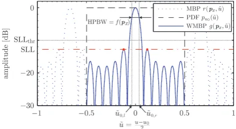
Fig. 7. Modified beam pattern (MBP)r(px,u)˜ , beta PDFpu0(u)˜
(ub=0.5, a=1), weighted modified beam pattern (WMBP)
g(px,u)˜ with marked half-power beam width, which is used as
ob-jective functionf (px)for array geometry optimization.
WMBP below a threshold SLLthr. Thus, the array geometry optimization results in the constrained minimization problem min
px
f (px), s.t. SLLg(px,u)˜ ≤SLLthr. (15) Figure 7 exemplarily illustrates the calculation of the ob-jective function for the already mentioned 8-element ULA with sensor spacing 34λ. At first, the product of the MBP and the PDF provides the WMBP, following (Eq. 13). Here, we use the beta PDF from (Eq. 8) withub=0.5 anda=1. Note that the SLL of the WMBP (SLL= −12.8dB) is be-low the threshold SLLthr= −10dB. Therefore, the HPBW of the WMBP is calculated using equation (Eq. 14) with f (px)= ˜u0,r− ˜u0,l.
3.2 Optimization results
Three exemplary results of the geometry optimization will now be presented in order to illustrate the accuracy of the proposed objective function in conjunction with the evolu-tion strategy. The DOA estimaevolu-tion performance for one sig-nal in terms of the mean squared error (MSE) is evaluated for each generated geometry and compared to the standard ULA. The target’s DOAu0 is chosen to underlie the beta PDF, whose parameters are specified in the respective ex-ample. For DOA estimation, we use the WDML estimator from (Eq. 12) withα=5, i.e., a high influence of the prior compared to the Maximum a posteriori estimator is consid-ered. Each of the MSE curves is based on 6·104Monte Carlo runs per SNR simulation point. The number of snapshots is K=10 and we consider array geometries withN=8 sensor elements. The respective optimized array geometries, includ-ing the standard ULA, are shown in Fig. 8.
In addition, the MSE performance plots also include the asymptotic variance
σDML2 = 1
2π2N U 1 SNR
1+ 1
N 1 SNR
Fig. 8. ULA (a) and optimized array geometries with respect to (b) example 1, (c) and (d) example 2 and (e) example 3.
of the DML estimation error with the signal-to-noise ratio defined in (Eq. 2) and the variance of the element positions
U= 1 N
N X
n=1
px,n− 1 N
N X
m=1 px,m
!2
(17)
(Athley, 2005) and (van Trees, 2002). Note that in the single signal case, (Eq. 16) is identical to the Cram´er-Rao lower bound for a stochastic signals(k)(Stoica and Nehorai, 1990).
3.2.1 Example 1
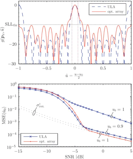
We choose the beta PDF with ub=1 and a=1, i.e., the DOA estimation should be unambiguous for the half space
−1≤u≤1. In addition, the SLL threshold is set to SLLthr=
−10dB. The optimized geometry is shown in Fig. 8b). Fig-ure 9 plots the WMBP of the standard ULA and the opti-mized array. It can be seen that the ULA provides (near) ambiguous DOA estimates for| ˜u|>0.9. The optimized ar-ray, however, is unambiguous for the complete half space and exhibits a reduced HPBW at the expense of a slightly in-creased SLL. The associated DOA MSE curve is presented in the bottom of Fig. 9. It can be clearly seen, that in the case ofub=1, i.e. a uniform distributed DOAu0∈ [−1,1], the optimized array significantly outperforms the ULA due to the effect of outliers. If the ULA’s ambiguous regions are not taken into account, i.e.ub=0.9, its asymptotic MSE im-proves, but still does not reach the optimized array due to the marginal difference of the beam widths. Furthermore, Fig. 9 also shows, that the WDML estimator asymptotically approaches the asymptotic variance of the DML estimator, as it has been defined in (Eq. 16).
3.2.2 Example 2
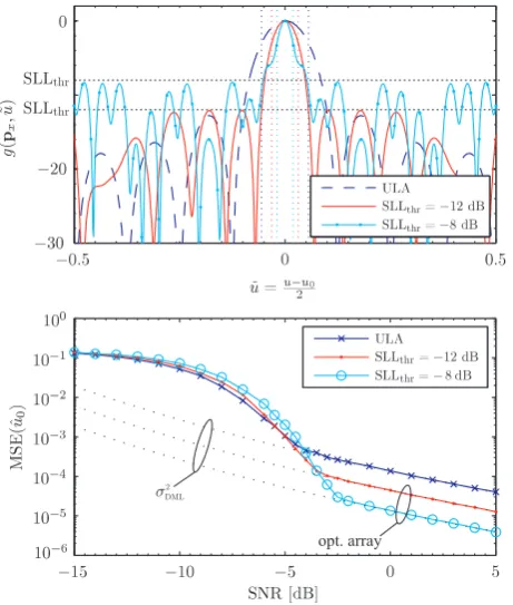
In this example, we assume that the signal’s DOA is limited to−0.5≤u0≤0.5. Therefore, we choose the beta PDF with
Fig. 9. Top: WMBP for example 1 for the standard ULA and the optimized array. Bottom: DOA MSE performance of the WDML estimator for example 1 for a single signal. The DOAu0follows
the PDF from (Eq. 8) withub=1 andub=0.9, respectively, and
a=1.
ub=0.5 anda=1 (see Fig. 5). To avoid ambiguities inside this region, the SLL is bounded above to SLLthr= −12dB and SLLthr= −8dB, respectively. The optimized geometries are shown in Fig. 8c) and d). Figure 10 plots the WMBP’s for the ULA and the two optimized arrays. Due to the re-duced DOA region, ambiguities outside of−0.5≤u0≤0.5 can now be accepted, as they have no impact on DOA esti-mation. This allows for an increased array aperture which leads to a smaller HPBW. The MSE curves in Fig. 10 show an improvement in terms of the SNR in the asymptotic re-gion of 5dB and 10dB, respectively, compared to the ULA.
3.2.3 Example 3
Fig. 10. Top: WMBP for example 2 for the standard ULA and the optimized arrays. Bottom: DOA MSE performance of the WDML estimator for example 2 for a single signal. The DOAu0follows
the PDF from (Eq. 8) withub=0.5 anda=1.
4 Conclusion
In this paper, a novel method of array geometry optimization with the aim of DOA estimation improvement has been pre-sented. Based on a modification of the standard beam pattern and an angular a priori density function, an objective function has been derived. By controlling the beam width and the SLL of the modified beam pattern, the MSE curve of DOA esti-mation is affected, while ambiguities are avoided. By the use of the a priori PDF, we have demonstrated, how effects from the “real world” like the DOA’s statistical properties, antenna characteristics like the element factor and the transmit beam pattern or hardware constraints like radomes or blinds can easily be taken into account in the optimization process. Us-ing an evolution strategy, we have presented four optimum array geometries and evaluated their DOA estimation perfor-mance. Compared to the standard ULA, it has been shown, that the MSE can be significantly improved.
Fig. 11. Top: WMBP’s for example 3 for the standard ULA and the optimized array. Bottom: DOA MSE performance of the WDML estimator for example 3 for a single signal. The DOAu0follows
the PDF from (Eq. 8) withub=0.75 anda=1.2.
References
Athley, F.: Threshold region performance of Maximum Likelihood direction of arrival estimators, Signal Processing, IEEE Transac-tions on, 53, 1359–1373, doi:10.1109/TSP.2005.843717, 2005. Gershman, A. B. and B¨ohme, J. F.: A note on most favorable array
geometries for DOA estimation and array interpolation, Signal Processing Letters, IEEE, 4, 232–235, doi:10.1109/97.611287, 1997.
Krim, H. and Viberg, M.: Two decades of array signal process-ing research: The parametric approach, IEEE Signal Processprocess-ing Magazine, 13, 67–94, 1996.
Oktel, U. and Moses, R. L.: A Bayesian approach to array geome-try design, Signal Processing, IEEE Transactions on, 53, 1919– 1923, doi:10.1109/TSP.2005.845487, 2005.
Richmond, C. D.: Mean-squared error and threshold SNR predic-tion of Maximum-Likelihood signal parameter estimapredic-tion with estimated colored noise covariances, Information Theory, IEEE Transactions on, 52, 2146–2164, doi:10.1109/TIT.2006.872975, 2006.
Stoica, P. and Nehorai, A.: MUSIC, Maximum Likelihood, and Cram´er-Rao bound, Acoustics, Speech and Signal Process-ing, IEEE Transactions on, 37, 720–741, doi:10.1109/29.17564, 1989.