International Journal of Engineering
J o u r n a l H o m e p a g e : w w w . i j e . i rModeling of the Capacitated Single Allocation Hub Location Problem with a
Hierarchical Approch
M. Karimia, A. R. Eydib, E. Korani*b
a Department of Industrial engineering, Najafabad Branch, Islamic Azad University, Isfahan, Iran b Department of Industrial engineering, University of Kurdistan, Sanandaj, Iran
P A P E R I N F O
Paper history: Received 29 April 2013
Received in revised form 13 July 2013 Accepted 22 August 2013
Keywords:
Hierarchical Hub Location Capacitated P-hub Median
A B S T R A C T
The hierarchical hub covering facility location problems are applied to distribution systems, transportation, waste disposal, treatment services, emergency services and remote communication. The problems attempt to determine the location of service providers' facilities at different levels and specify their linking directions in order to reduce costs and to establish an appropriate condition in distribution network. By utilizing these problems, the present paper attempts to allocate "capacitated" option to each provider service and consequently establish and choose the best possible condition, so that demands centers are rationally and effectively guided by service providers' centers and their request never remains without response. To do this, the model "the capacitated single allocation hierarchical hub median location problem" is developed, created and provided. In addition, considering of the increasing demand, modulating choices are addressed in order to fulfill the future needs and to impose uncertainty in decision making in the results. To validate the model, we used IAD data, which the results confirm its consistency.
doi:10.5829/idosi.ije.2014.27.04a.08
1. INTRODUCTION1
Hub location problems attempt to consider hub locating and to allocate demand nods to created hub facilities. In a single allocation P-hub median problem, among potential hub nodes, P-hub frequency is chosen and each demand point (non-hub nodes) is exactly allocated to a single hub. They mainly aim to reduce routing costs and to minimize the cost of hubs' establishment. The number of the hub nodes (e.g. P) is already determined and the hubs are directly linked. This problem has a finite space and a discrete structure. Its application is summarized in two general domains transportation and communication. O'kelly [1] first provided p-hub location problem as a mathematical model by studying airline networks. Campbell [2] provided the first mathematical formulation for single allocation P-hub median problem, and then a few years later presented a linear model for solving P-hub locating problem in a network with N node. Skorin-Kapov et al. [3] presented a new mixed integer formulation for this problem. Ernst
*Corresponding Author Email: [email protected] (E. Korani)
and Krishnamoorthy provided another different integer linear formulation for solving larger problems which needed less constraints and variables. In addition, it was shown that how Australian Post Office uses different values of α discount for distribution and collection network [4]. To further study, Campbell's [5] and Alumur and Kara's [6] works are suggested. Hierarchical hub problems are one issue raised in the hub location problem.
Chen et al. [7] examined the strategic design of delivery networks which could efficiently provide these services. Because of the high cost of direct connections, they focused on tree-structured networks and established the complexity of the problem. They also exploited an empirically identified solution structure to create new neighborhoods which improved solution values over more general neighborhood structures.
Labbe and Yaman [8] considered the problem of locating hubs and assigning terminals to hubs for a telecommunication network. The hubs were directly connected to a central node and each terminal node is directly connected to a hub node. Their aim were to minimize the cost of locating hubs, assigning terminals
and routing the traffic between hubs and the central node. They presented two formulations and showed that the constraints are facet-defining inequalities in both cases.
Wagner [9] proposed new model formulations for hub covering problems and it was improved. This model discussed multiple and single allocation problems, including non-increasing quantity-dependent transport time functions for transport links for the latter case.
Yoon and Current [10] introduced a new hub location and network design formulation that considered the fixed costs of establishing the hubs and the arcs in the network. In addition, the variable costs associated with the demands on the arcs. The problem was formulated as a mixed integer programming problem embedding a multi-commodity flow model [10]. Alumur and Kara [11] focused on cargo applications of the hub location problem. They proposed a new mathematical model for the hub location problem that was relaxed the complete hub network assumption. Their model minimized the cost of establishing hubs and hub links and formulated a single-allocation hub covering model that permuted visiting at most three hubs on a route [11]. Alumur et al. [12] provided a uniform modeling treatment to all the single allocation variants of the existing hub location problems, under the incomplete hub network design. So that, they defined the single allocation incomplete p-hub median, the incomplete hub location with fixed costs, the incomplete hub covering, and the incomplete p-hub center network design problems [12]. Calik et al. [13] studied the single allocation hub covering problem over incomplete hub networks and proposed an integer programming formulation. The aim of their model was to find the location of hubs. The hub links to be established between the located hubs and the allocation of non-hub nodes to the located hub nodes such that the travel time between any origin–destination pair was within a given time bound. They presented an efficient heuristic based on tabu search and test the performance of their heuristic on some well-known data sets. Campbell [14] provided time definite models for multiple allocation p-hub median problems and p-hub arc location problems. Service levels were imposed by limiting the maximum travel distance via the hub network for each origin– destination pair. Contreras et al. [15] considered the tree of hub location problem and proposed a four index formulation which yields much tighter LP bounds than previously proposed formulations.
Ernst et al. [16] studied the uncapacitated hub center problems with either single or multiple allocation. Both problems were proved to be NP-hard. So, they presented the integer programming formulations for both problems and proposed a branch-and-bound approach for solving the multiple allocation case [16]. Limbourg and Jourquin [17] were used from a set of estimated potential locations as input for an iterative procedure
based on the p-hub median problem that took the variation in trans-shipment costs according to the number of trans-shipped containers into account [17]. Meyer et al. [18] presented an exact 2-phase algorithm where in the first phase, and computed a set of potential optimal hub combinations used a shortest path based branch and bound. They developed a heuristic for the single allocation p-hub center problem based on an ant colony optimization approach [18]. Sim et al. [19] presented the stochastic p-hub center problem with chance constraints, which they used to model the service-level guarantees. Contreras et al. [20] presented the Tree of Hubs Location Problem. It was a network hub location problem with single assignment where a fixed number of hubs have to be located, with the particularity which it was required that the hubs were connected by means of a tree. The problem combined several aspects of location, network design and routing problems. They proposed an integer programming formulation for the problem [20]. Lin [21] studied the integrated hierarchical hub-and-spoke network design problem for dual services. It integrated otherwise mutually exclusive secondary route networks for their respective services so that the total operating cost was minimized while meeting the service time and operations restrictions. A directed network configuration and formulate a link-based integer mathematical model was proposed [21]. Meng and Wang [22] developed a mathematical program with equilibrium constraints (MPEC) model for the intermodal hub-and-spoke network design (IHSND) problem with multiple stakeholders and multi-type containers. Their model incorporated a parametric variational inequality (VI) that formulated the user equilibrium (UE) behavior of intermodal operators in route choice for any given network design decision of the network planner. In addition, this model used a cost function that was capable of reflecting the transition from scale economies to scale diseconomies in distinct flow regimes for carriers or hub operators [22]. Yaman [23] studied allocation strategies and their effects on total routing costs in hub networks. Given a set of nodes with pairwise traffic demands, the p-hub median problem was the problem of chosen p nodes as hub locations and routing traffic through these hubs at minimum cost. This problem had two versions; in single allocation problems, each node could send and receive traffic through a single hub, whereas in multiple allocation problems, there was no such restriction and a node might send and receive its traffic through all p hubs. Furthermore, models for variations of this problem with service quality considerations, flow thresholds, and non-stop service was presented [23].
transportation costs, modal connectivity costs, and fixed location costs under service time requirements. A tabu search meta-heuristic was used to solve large size (100 nodes) problems.
Alumur et al. [25] introduced the multimodal hub location and hub network design problem. They approached the hub location problem from a network design perspective. In addition, to the location and allocation decisions, they also studied the decision on how the hub networks with different possible transportation modes must been designed. In this multimodal hub location and hub network design problem, they jointly considered transportation costs and travel times, which were studied separately in most hub location problems presented in the literature. They first proposed a linear mixed integer programming model for this problem and then derive variants of the problem that might arise in certain applications.
Alumur et al. [26] discussed about of Hierarchical multimodal hub location problem. This paper deals with time bound deliveries between pair origin-destination, so that they ensured each demand give the service in the time bound. In addition, they showed that the locations of airport hubs was less sensitive to the cost parameters compared to the locations of ground hubs and it was possible to improve the service quality at not much additional cost in the resulting multimodal networks [26].
Elmastas [27] first observed a three-level cargo delivery network in Turkey and modeled its three-level structure in a hub median problem in order to minimize the cost of hubs establishment. In Elmastas’s paper, two types of hub facilities are presented, so that, they performed their activities in a network with three level structure. Each level of network include some demand nodes and hub facilities, where the first level links central hubs with a complete network, the second level assigns remaining hubs to the central hubs through star networks and the third level joins the demand nodes to the hubs with star networks [28]. Then, Yaman [28] developed the model and considering the objective function of routing cost rather than establishment cost, developed single allocation P-hub median problem (SA-TH-HM). In addition, by creating a complete network linking between first level hubs, Elmastas star model was converted into a complete network structure [28]. The hub location problems can be divided into two main parts, capacitated and non-capacitated. In the literature on single allocation hub locating problems, the capacitated structure of service providers' centers and their links is considered to create a more realistic situation. Alumur et al. [6] classified and surveyed the network hub location models. They introduced some recent trends on hub location and provided a synthesis of the literature [6]. They also observed that the capacitated hub location problem has two well-known structures: single allocation and multiple allocations.
They differ in how non-hub nodes are allocated to hubs. In single allocation, all the incoming and outgoing traffic of every demand center is routed through a single hub; in multiple allocations, each demand center can receive and send flow through more than one hub [6].
There are many papers for the single allocation capacitated hub location problem, some of them as follow; the first linear integer formulation for the single allocation capacitated hub location problem presented by Campbell [2].
Aykin [29] introduced the new version of the capacitated hub and spoke network problem with objective function of fixed charge costs. Then, the lower bounds are obtained by lagrangean relaxation, and presented a branch-and-bound algorithm to solve it [30]. Jaillet et al. [30] designed capacitated hub location models for airline networks. They proposed three basic integer linear programming models, each corresponding to a different service policy and presented heuristic schemes based on mathematical programming [30].
Ernst and Krishnamoorthy [31] presented two new formulations for the capacitated single allocation hub location problem. Their formulations are a modified version of the previous mixed integer formulations developed for the p-hub median problem [31].
Labbe´ et al. [32] investigated some polyhedral properties of the single allocation capacitated hub location problem and developed a branch-and-cut algorithm based on these results.
A different approach to the capacitated single allocation hub location problem is presented by Costa et al. [33]. They are introduced two bi-criteria single allocation hub location problems: in a first model, total time is considered as the second criteria and, in a second model, the maximum service time for the hubs are minimized [33].
Tavakkoli et al. [34] presented a novel multi-objective mathematical model for capacitated single allocation hub location problem and solved it by a multi-objective imperialist competitive algorithm (MOICA). Finally, to prove its efficiency, the related results are compared with the results obtained by the well-known multi-objective evolutionary algorithm, called NSGA-II [34]. However, this model has been designed for one level of service, too.
solution method with Lagrangian relaxation bounding strategy, and report some results of numerical experiments using real aviation data [36].
Boland et al. [37] suggested a new formulations and solution approaches for multiple allocation hub location problems. They employed flow cover constraints for capacitated problems to improve computation times [37].
Yaman [38] studied the uncapacitated hub location problem with modular arc capacities. Then, Yaman and Carello [39] extended Yaman’s [38] model, and the amount of traffic passing through the hub specified as a hub’s capacity.
There are many papers in the capacitated hub location literature, but all of them are designed for systems with one level of services. So, this paper presents a new model with more than real situation in the world. Many hub location problems are designed for transportation system, cargo delivery systems, telecommunication network system, production-distribution systems and etc. [6]. However, all of them have been noticed by one level of services. Another hand, regarding the applied field of the hierarchical problem, the following cases could be mentioned: Solid waste management systems, Production-distribution systems, Education systems, Emergency medical service (EMS), Telecommunication network systems, Cargo delivery, Health care systems and other relevant ones above are examined by Sahina and Sural [40] which is a comprehensive research on hierarchical problems. Nevertheless, the capacitated hub location problems are designed without hierarchical structure for the hierarchical systems in the real world. Thus, we designed a new single allocation capacitated hub location problem with a nested hierarchical structure to be closer to the real situation.
Single allocation hub location problem in which hubs become capacitated are identified as capacitated single allocation hub locating problem (CSAHLP) with one level of service. Campbell [28] presented a mixed integer primary linear programming for CSAHLP. Ernst and Krishnamoorthy [31] extended the formulation presented by Kapov et al. [3] for problem's capacitated and non-capacitated version. They also presented a new mix integer linear programming (MILP) formulation which is an adaptation of CSAHLP related to the formulation by same authors for the non-capacitated hub median problem. Labbe et al. [32] conducted CSAHLP by imposing capacity on the flow links passing each hub and proposed a branch-and-bound algorithm. Yaman and Carrello [39] investigated hub location problem with modular link capacities. Only the implementation cost in problem was considered. In addition, in a study by Yaman [41], hub locations and links were identified to reduce costs in hub median problem with regard to capacity for arcs. He also considered two formulations and an innovative
algorithm for solving problem in which the solving methods quality was compared. Correia et al. [42] revised and modified one of the most famous formulations presented in the literature on capacitated single allocation hub location problem. Presenting an example, they showed that the old formulation in the balance limitations (constraints) balance suffers from some disadvantages. Therefore, by adding cut constraints, they concluded that their formulation plays a critical role in imposing properly capacity conditions on the base problem and also it helps to reduce solution time. In the literature of the hierarchical, hub location problems are not significantly considered about of capacity. As a result, Yaman and Elloumi's [43] contribution is as the last work on this issue presented two hierarchical problems and focused on the quality of services rather than the capacity. They mainly attempted to reduce the length of the longest route and to minimize total routing cost. However, the present paper attempts to combine the hierarchical hub location problem and the capacitated hub problem. Of course, the model design has been in a manner that with the smallest variations in the costs of network establishment and solving times, it has been achieved to the optimal result, which the results are more close to real conditions of the world. These conditions allocate demand nodes to service provider facilities in a manner that they do not encounter a non-responding state at different levels and a minimized total cost is achieved. The main novelties of our works are mention as follow:
1) We attempted to combine the hierarchical hub location problem and the capacitated hub location problem. Because, many companies and complex systems are used the hierarchical structure in their activities; so, we tried to create a new model for this real situation.
2) Our model is one type of the capacitated hub location model, but the capacitated hub location models with one level of service are revised and modified in the literature by Correia et al. [42]. Thus, we extended Correia’s idea from “the capacitated single allocation hub location problem with one level of service” to “the capacitated single allocation hub location problem with the hierarchical structure”.
In order to achieve this, this paper presents the capacitated single allocation hub location problem in section 2. Section 3 presents the computational results of the model using Iranian Airport Data (IAD) in order to confirm the performance of the proposed model. The results of the present study and future research are presented in section 4.
2. PROBLEM FORMULATION
in a realistic situation where different levels of services have been considered for transportation network.
In this section, a mixed-integer programming formulation for the problem with three-index (three-attribute) variables is presented. Among the works on revision of classic P-hub problem with single index characteristics, O'kelly [1] study with binary quadratic model could be mentioned. Afterwards, some works have been done by Campbell [2] and Skrin-Kapov [3]. They presented linear models with 4-index variables.
Then, Ernst and Krishnamoorthy [4] created a multi-commodity flow model with three-index variables, which each origin of a single commodity flows along the network direction. A model based on three-index variables was developed in order to minimize routing cost [28]. The current work attempts to present model hypotheses, relevant parameters, indices and decision making variables to develop the Capacitated Time Restricted Hierarchical Hub Median Poblem With Single Assignment (SA-TH-CHM). The symbols are specified as follows:
I is the demand points, HÍI is potential points for generating second level service providing hubs, and
H
CÍ is potential points for first level service providing central hubs. PH and PC specify the number of hubs and
central hubs to be generated, respectively. Fij specifies exchanges from node iÎIto jÎI. Normally, the flow from a node to itself is equal to zero (i.e.Fii=0;"iÎI). It is assumed in the model that Fii=0 works for alliÎI.
ij
C is the routing cost of a unit of flow from node iÎI to jÎI. In the model, Cij=Cji works for all pair nodes i and j and alsoCii=0, iÎI. aH and aC are reduction factors and their value always ranging zero and one, in the case aH ³aC [28]. aHand aC are the discount coefficients for route generation cost between hubs and central hubs and high level hubs. If node iÎI is allocated to hub jÎH and hub j is allocated to central hublÎC, then variable xijl is equal to 1, otherwise is equal to zero. wi
jl is the traffic demands between hub
H
jÎ and central hub lÎC, due to node iÎI as origin or destination. vi
jlspecifies exchanges rate passing central
hubkÎCto central hub lÎC\{k}, due to iÎIas origin.
tij is the passing time from node iÎI to node jÎI, and
ji
ij t
t = , also tii=0. It is possible to make the duration of movement between hubs, central hubs and two central hubs shorter because more advanced and special vehicles could be used. This is possible by discount factors aH andaC. The value of these parameters are limited to (0, 1) and aH³aC. The following variables could be defined by the Wagner's extended idea [2]: If
C
lÎ , then Dˆlshows the time when all the flows caused
by demand nodes and hubs allocated to the central hub l
reach the node l. Dl shows the time when vehicles toward the demand nodes and their hubs linked to the central hubs l, leave l for destination. With these variables, it is possible to define cargo delivery upper limit with determined time bound of b for the problem as follows. For eachi Î I , then TFi calculates all
exchanges from node i to other points (i.e. I
i TF
F i
I m
im= " Î
å
Î
; ).
For each iÎIif it is selected as hub, its service capacity for the first and second levels are shown by Gci andGhi, respectively. If xlllfor eachlÎC is equal to 1, it could be said that central hub is established in the node, and also if xjjlfor each jÎH,lÎCis equal to 1, it could be said that the second level hub is established. According to the above, the problem is as follows.
2. 1. Objective Function The Equation (1) shows the objective of this problem which is equal to total routing costs due to exchanges between their relevant hubs, hubs, and central hubs, and also exchanges between central hubs themselves.
åå å
å å å å
å åå
Î Î Î
Î Î Î Î
Î Î Î
+
+ +
=
I
i jClC j jl
i jl C
I i jHlC j
jl i jl H C
l ijl H j
ij I
i
ri I r
ir
v C
w C x
C F F z
} \{
} \{
) ( min
a
a (1)
2.2. Hierarchical Hub Location Equations Equation (2) guarantee that each demand node is allocated to one hub and one central hub. Equation (3) show that if node i links to hub j and central hub of l, then node j must be a hub linked to the central hub l. Equation (4) guarantees if node j is allocated to the central hub l, then l becomes necessarily central hub. The number of hubs and central hubs are specified by
H
P and PC, respectively, which these Equations are mentioned in Equations (5) and (6).
I i x
H j l C ijl
Î " =
å å
Î Î
1 (2)
C l i H j I i x
xijl£ jjl "Î , Î \{}, Î (3)
} { \ ,l C j H
j x x lll H
m jml
Î Î " £
å
Î
(4)
å å
Î Î = H
j
H C
l
jjl p
x (5)
C C l
lll p
x =
å
Î
If node i is linked to a hub which in turn it is linked to central hub i, then traffic happens from node i to the nodes which are linked to other central hubs and leave the node. If node i is not linked to central hub l, traffic happens from node i to the nodes which are linked to the central hub i and move toward the node. These flows are assumed in Equations (7) and (12). In Equation (8) (i.e. cut equations) which is taken from Correia's idea [42], an upper bound for traffic volume between the hub and the central hub, and the central hub with another the central hub are considered. Equation (8) gives a complete description of capacitated problem. In fact, considering these equations in the model formulations, variables i
lk
v are allowed to be contrary to zero, regardless ofxijl=0. The Equation (8) are actually
a preventing action to this problem.
In Equations (9) and (11), amount of wijl is
determined by allocation variables. Traffic in proximity of node i and between hub node j and central node l, is the same traffic between node i and the nodes which are linked to hub j. In this case, node i is linked to hub j and central hub l, otherwise amount is zero. Note that the traffic between nodes i and j will not be happened from hub j toward the central hub l, when i links to j. The Equation (10) is for modification of LP. Constraints 13 enable the presence or the absence of three-level allocations.
C l I i x x F v
v
H j ijl rjl I
r ir I
C k
kl i l
C k
i
lk -
å
=å
å
- " Î Îå
Î Î Î
Î
, )
(
} { \ } {
\ (7)
C l I i x F v
I
m im j H ijl
k l C k
i
lk £
å
å
" Î Îå
Î Î
¹ Î
,
, (8)
} { \ , , ) ( ) (
} { \
j C l H j I i x x F F
w ijl rjl
j I r
ri ir jl
i ³
å
+ - "Î Î ÎÎ (9)
} { \ ,
0 j H l C j
xljl = " Î Î (10)
C l H j I i
wijl³0 " Î , Î , Î (11)
} { \ , ,
0 i I k Cl C k
vikl³ " Î Î Î (12)
C l H j I i
xijl Î{0,1} " Î , Î , Î (13)
2. 3. Capacity Equations In this model, Equation (14) specifies the maximum ability for estimating second level demands for each location jÎH which is sameGhj, i.e. the capacity for providing services of second level in location j. Equation (15) for each location lÎCdetermines maximum ability for estimating
first level demands which is sameGcl, i.e. the capacity for providing first level services in location l.
H j h x
TF j
C
l iI
ijl
i £G " Î
åå
Î Î (14)
C l c x f
TF l
H
j i I
ijl ij
i- £G " Î
åå
Î Î
)
( (15)
2. 4. Time Bound Equations In case node i links to the central hub i, then it will be directly linked to a hub group j, which it will be also linked to central hub l. Equation (16) estimated all travel time of traffic demand of node i toward the central hub l, then the outcome puts into itsDˆl. Equation (17) computed the movement time of flow traffic between two central hubs and then insert into its Dl. In addition, in case lÎC and kÎC\{l}،
k
l D
D ³ ˆ always work. For the travel time of traffic at
each origin arrives to destination at the maximum time of β, the model uses from Equation (18). Equation (19) is not-negative makers.
C l I i x t t
D ij H jl ijl
H j
l ³
å
+ " Î Î Î, )
(
ˆ a (16)
C k C l x
t D
Dl ³ ˆk +aC kl kkk " Î , Î (17)
C l I i x
t t
D ji ijl
H j
lj H
l+
å
+ £ " Î Î Î, )
(a b (18)
C l D
Dˆl ³0, l³0 " Î (19)
A problem description has been presented by an example that has a node set with n=7 and have been showed the outputs of the problem whereas PH=3 and
PC=1. The input node set of the example and the
resulting network of the model are displayed in Figures 1 and 2, respectively. According to this solution, x175=
x275=x775=x355=x665 = x465 =1 so the nodes of 5, 6 and 7
are chosen as hub nodes andalso x555=1. Therefore, the
node of 5 is selected as central hub node. The notations of flow balance Equation (9) for nodes i=4, j=6 and l=5 are (f41+f14)(x465 – x265) + (f42+f24)(x465 – x265) +
(f43+f34)(x465 – x365)+ (f45+f54)(x465 – x565) + … +
(f47+f74)(x465 –x765)≤ w465. On the other hand, the below
symbolizations are capacity constraints for all hubs and central hub nodes, and the time bound constraints for the route between node 2 and node 4. The capacity equations are TF4.x465 +TF6.x665 ≤Gh6, TF1.x175
+TF2.x275 +TF7.x775 ≤Gh7 and (TF1-f17).x175 + (TF2
-f27).x275 + (TF4-f46).x465 + TF7.x775 +TF3.x355 +TF6.x665 ≤
5
c
G . The time bound equations contain (t27+αHt75) x275 ≤
5
ˆ
Figure 1. The node set with n=7.
Figure 2. The output network of the model with n=7, PH=3
and PC=1.
3. RESULTS AND DISCUSSIONS
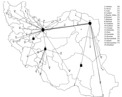
The Iranian Airport Data (IAD) was introduced by Karimi [44]. It includes the distances, costs, weights, capacities and fixed charge hub costs based on the hub airport location between 37 iranian cities. We assumed all the nodes as the demand set I, and we partitioned the 17 populous cities with maximum traffic among of facilities as a potential set of hubs (i.e., set of H) similar to Yaman [28] on Turkish network Data set. There are 10 populous cities in set of H, that their capacity were more than summation of all traffic; so, we chose them as a potential set of central hubs (i.e., set of C). In the next subsections, we presented the computational results and discussions on the IAD data for the model. Figure 3 shows the iran’s map with 37 nodes of it. The potential nodes of central hubs and hubs are characterized by square and circle, respectively.
In order to examine the cost trends with regard to number of pre-imposed central hubs, the problem was solved with both its new and old structure. Firstly, SA-TH-CHM model with capacity and cut equations and then Time Restricted Hierarchical Hub Median Poblem With Single Assignment (SA-TH-HM) without any constraints were implemented in order to investigate the effect of capacity and cut equations in the problem. Considerable changes were observed by comparing the results. The number of hubs was assumed to be 5 and central hubs in 5 different performances were assumed to be constant from 1 to 5 (i.e.,pCÎ{1,....,pH}). In addition, according toaC£aHandaC£aH, the magnitudes of discount coefficients in all calculations for pCÎ{1,....,pH}are considered to be aH =aH =0.9 andaC =aCÎ{0.9,0.8} .
3. 1. Graphical Reports As seen the models outputs results in Tables 1 to 6, overview for some outcomes in Figures 4 to 7, of course, the capacitated
hierarchical structure has taken advantage of more significance than its past structure, i.e. by increasing the central hubs from 1 to 5, two models SA-TH-HM and SA-TH-CHM show similar results in terms of the hub and the central hub facilities location.
Thus, this mentions above are confirmed it. Mostly, when PC=5, the location of the central hubs in both
models becomes exactly the same. However, by decreasing number of the central hubs in each stage of solving direction, the changes and also the differences between location of the hubs and the central hubs in the model output become increasingly higher, so that in the stat(aH,aC,aˆH,aˆC)=(0.9,0.8,0.9,0.8),
b
=2990andPC=1 in SA-TH-CHM, the 28 city and the 10-15-23-28
cities are selected as the central hub and the hubs, respectively.
In the same situation, the SA-TH-CHM model also choose the central hub and hubs at the 10 city and the 2-10-14-31-35 cities, respectively. Therfore, these outcome shown that more than 80% of the network structure has changed.
Figure 3. The map for IAD with n = 37, 17 and 10 number of
potential nodes for hubs and central hubs, respectively.
Figure 4. Grafical Veiw of hubs and central hubs locations in
the SA-TH-CHM, with IAD data, when β=2990,
) ˆ , ˆ , ,
(aH aC aH aC = (.9,.8,.9,.8) andPC=2.
1
2
3
5
4
6 7
1
2
3
5
4
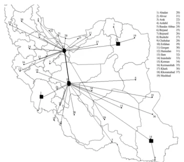
Figure 5. Grafical Veiw of hubs and central hubs locations in
the SA-TH-HM, with IAD data, when β=2990,
) ˆ , ˆ , ,
(aH aC aH aC = (.9,.8,.9,.8) and PC=2.
Figures 4 and 5 show the outputs of the two models
SA-TH-CHM and SA-TH-HM, when (aH,aC,aˆH,aˆC)
0.8) 0.9, 0.8, (0.9,
= ,PC=2 and β=2990, respectively. In
addition, Figures 6 and 7 show the outputs of
SA-TH-CHM and SA-TH-HM, when
0.9) 0.9, 0.9, (0.9, ) ˆ , ˆ , ,
(aH aCaH aC = , PC=2 and β=2990,
respectively.
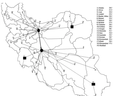
In these figures, square symbol indicates the hubs node and rectangle indicates the central hubs. In Figure 4, more logical state than Figure 5 could be observed. Of course, there are some similarities between these two figures; for example, city 31 in each figure is selected as a central hub which covers northern and western north area. Despite this similarity, the second central hub is selected in a more significant distance than the first significant model in Figure 4 which is the result of SA-TH-CHM. In Figure 4, the distance between two facilities at the first levels is more than the distance between the hubs and the central hub, which it is more logical because the provision capacity and services variety of the facilities increases by an increase in their level. Of course, these states could be confirmed and known by assuming that
a
C£
a
H[28]. On the other hand, if we divided vertically Figures 4 as the output of SA-TH-CHM model, the central hubs are located in two different sides, in which situation of fair distribution for the service provider's facilities are fulfilled. However, Figure 5 is results of SA-TH-HM model, if it separated into sections left and right from the middle by a vertical cut. Both of the central hubs will be also located in the left side. Thus, it is not fair situation for service delivery. The other significant difference in SA-TH-HM model opposite of SA-TH-CHM model is that demand nodes are allocated to hubs and central hubs with a long distance. However, this is rarely seen in SA-TH-HM model.For example in the Figure 5 which is output of SA-TH-HM model, demand nodes 36, 35, 5 and 6 are
located with a far distance from the hub, which do not indicate a fair distribution . In addition, the hub nodes in the output of SA-TH-HM model provide services at least for two demand nodes; but, in the Figure 4 which is a output of SA-TH-CHM, the central hub located in the node of 10 covers more than 6 demand nodes. In addition, Figures 5 and 7 confirm that hubs in SA-TH-HM provide less services for demand nodes, in which, location of the hubs have been not significant. In SA-TH-HM in both Figures 5 and 7, the hubs nodes of 2 and 14 provide services to only one of demand node and in other hubs (i.e., 23) second level of services provide only for two demand nodes. The establishment of these hubs is not practically necessary and only increases the costs.
In Figure 4, the SA-TH-CHM selected the 31 and 19 nodes as central hub that have been located in the north and northeast, when β=2990, (aH,aC,aˆH,aˆC)= (.9,.8,.9,.8) and PC=2, respectively. This is occur to
location of hubs have been change and chosen the 3, 10 and 19 nodes as hub, Such that, the central hubs have been away from each other. And the hubs have been nearby to their central hubs. In the event that, Figure 5 displayed unlike this status in illustrating by the SA-TH-HM. Figure 4 is a more logical structure than Figure 5 depicts for relation between hubs and central hubs, and central hubs together. In addition, relevance of among services facilities happened similar to above conditions in Figures 6 and 7.
3. 2. Effect of Capacity and Cut Equations on the Total Routing Cost
To better understand capacity situation on the base structure, Tables 1 and 2 are defined for the routing costs of TH-CHM and SA-TH-HM with different cases of discount coefficients, the number of the central hubs, different amounts of β
and the constant number of PH =5, respectively.
Figure 6. Grafical Veiw of hubs and central hubs locations in
the SA-TH-CHM, with IAD data, when β=2990,
) ˆ , ˆ , ,
Figure 7. Grafical Veiw of hubs and central hubs locations in
the SA-TH-HM, with IAD data, when β=2990,
) ˆ , ˆ , ,
(aH aC aH aC = (.9,.9,.9,.9) andPC=2.
The routing costs trends are presented in Figures 8, 9 and 10 by the graphical reports in the line charts. Figures 6 and 7 are depicted for the routing costs of the
models SA-TH-CHM and SA-TH-HM with equal
states, i.e. PC = 2, 3 and 4 with different types of time
bound (i.e., β), respectively. Figures 8 and 9 showed that with increasing the parameter of PC from 2 to 4,
both SA-TH-CHM and SA-TH-CHM had relatively equal costs and their variation trend is declining. Of course, by decreasing the number of central hubs in each variation stage, the routing costs will be more obvious, so that the routing cost in state
0.9)
0.9,
0.9,
(0.9,
)
ˆ
,
ˆ
,
,
(
a
Ha
Ca
Ha
C=
, β=2990 andPC=l in the SA-TH-CHM is 189.179506 and in the
SA-TH-HM the routing cost is 146.965061. In addition, the
routing cost in the state of
0.8)
0.9,
0.8,
(0.9,
)
ˆ
,
ˆ
,
,
(
a
Ha
Ca
Ha
C=
, β=3 and PC=3110 forthe SA-TH-CHM is 157.035483, while the routing cost in the SA-TH-HM model is 141.868391. The difference between these costs (i.e., 15.167092) is rational and indicates accuracy of the formulation; because, this cost difference is insignificant amount, opposite the capacity condition. Thus, it confirms the intelligent designing SA-TH-CHM. Figure 10 shows the routing costs of two models for particular states PCÎ{1,2,3,4,5}, β=∞ and
0.8) 0.9, 0.8, (0.9, ) ˆ , ˆ , ,
(aH aCaHaC = which confirm
above-mentioned suggestions. The costs have significant difference only in stringent state PC=l as a natural and
rationalized state, because the developed model has fulfilled capacity requirements in exchange for this difference. Notably, by imposing delivery time upper bound from 3110 to 2990 in the problem, the costs are increased considerably up to 0.22 percent.
3. 3. Effect of Capacity and Cut Equations on the Locations of Hubs and Central Hubs One of the
results of the present study is the location of hubs and central hubs which Tables 3 and 4 show the location of service providing location in different levels for the models SA-TH-CHM and SA-TH-HM with different states of discount coefficients PCÎ{1,2,3,4,5},
} ,
{2990,3110 ¥
Î
b and constant numbers PH=5,
respectively.
In order to see the effect of discount factors on facilities location in different levels and consequently the cost of transportation between the central hubs, the results from the states PC=2, (aH,aC,aˆH,aˆC)
0.8) 0.9, 0.8, (0.9,
= , β=2990 in both models were
investigated. Thus, we found that the routing cost of SA-TH-CHM has been 157.035483 and the central hubs location of cities 19 and 31 and the hubs of cities 31, 19, 15, 10 and 3 were selected. However, the routing cost of the model SA-TH-HM has been 141.868391, and cities 10 and 31 were regarded as the central hubs and cities 14, 23, 10, 31 and 2 as the hub nodes. It is seen that the developed model of SA-TH-CHMhas changed one out of two central hubs (i.e. change of city 10 to 19) under the specified states.
Figure 8. The routing cost of SA-TH-CHM for IAD for
different amount of β, PCÎ{2,3,4} and
0.9) 0.9, 0.9, (0.9, ) ˆ , ˆ , ,
(aH aC aH aC = .
Figure 9. The routing cost of SA-TH-HM for IAD for
different amount of β, PCÎ{2,3,4} and
0.9) 0.9, 0.9, (0.9, ) ˆ , ˆ , ,
(aH aC aH aC = .
142 144 146 148 150 152 154 156 158 160
2 3 4
Rou
tin
g
co
st
PC
2990 3110
∞
142 143 144 145 146
2 3 4
Rou
tin
g
co
st
PC
2990 3110
Figure 10. Compare the routing cost of SA-TH-CHM and
SA-TH-HM for IAD with β=∞,
0.9) 0.9, 0.9, (0.9, ) ˆ , ˆ , ,
(aH aC aH aC = and PCÎ{1,2,3,4 ,5}.
Figure 11. Compare the elapse times of SA-TH-CHM and
SA-TH-HM for IAD with β=∞,
0.8) 0.9, 0.8, (0.9, ) ˆ , ˆ , ,
(aH aCaH aC = and PCÎ{1,2,3,4 ,5}.
In addition, hubs 15, 19 and 31 are replaced with 23, 14 and 2. This trend is seen at most of the cases which shows the effect of the developed model on the main body of output network. In Table 3, city 31 is selected more than 85% of times as a central hub and city 10 more than 88% of times as a central hub.
In addition, city 31 in more than 96 % of times is selected as a hub, but city 10 in 100% of times is selected as a hub and when β=∞ and PC =1, city 31 is
selected as central hub in all examples and if PC= 2,
cities 31 and 10 are the central hubs. These two cities in Iran take privilege of efficient transportation systems, indicating the presence of a correct orientation in designing the SA-TH-CHM model.
3. 4. Effect of Capacity and Cut Equations on Computation Time In this section, the effect of different parameters on the CPU time is considered. The model has been performed by GAMS 21.7 and the solver CPLEX 11.0.0 on a 2.1 GH processor with core 2, RAM 4GB and a Windows 7. The calculation times of the unfeasible solutions are not presented. This
section is considered the effect of different amount of β
and discount coefficients on CPU time.
Information related to elapse time for SA-TH-CHM and SA-TH-HM on IAD data is shown in Tables 5 and 6, respectively. The increasing trend of CPU time due to decrease in the number of the central hubs could be observed in Tables 5 and 6. Furthermore, in 70% of different cases, elapse time in SA-TH-CHM model is more than run time of SA-TH-HM model, because capacity and cut equations are imposed into the SA-TH-CHM model. The maximum CPU times in SA-TH-CHM and SA-TH-HM models are 289.554 seconds and 124.353 seconds, respectively. On the other hand, the minimum elapse times in CHM and SA-TH-CHM are 2.376 and 1.527 seconds, respectively.
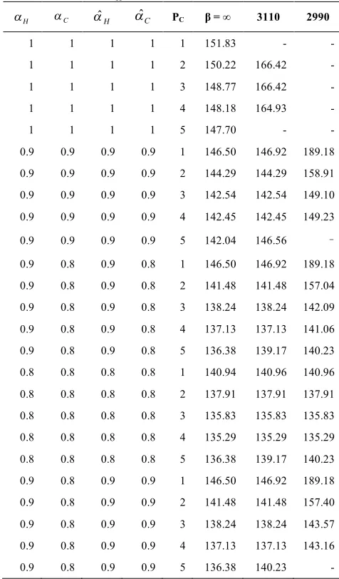
TABLE 1. Total routing cost of SA-TH-CHM for IAD data
with 37 nodes and PH=5
H
a aC aˆH aˆC PC β = ∞ 3110 2990
1 1 1 1 1 151.83 -
-1 1 1 1 2 150.22 166.42
-1 1 1 1 3 148.77 166.42
-1 1 1 1 4 148.18 164.93
-1 1 1 1 5 147.70 -
-0.9 0.9 0.9 0.9 1 146.50 146.92 189.18
0.9 0.9 0.9 0.9 2 144.29 144.29 158.91
0.9 0.9 0.9 0.9 3 142.54 142.54 149.10
0.9 0.9 0.9 0.9 4 142.45 142.45 149.23
0.9 0.9 0.9 0.9 5 142.04 146.56
-0.9 0.8 0.9 0.8 1 146.50 146.92 189.18
0.9 0.8 0.9 0.8 2 141.48 141.48 157.04
0.9 0.8 0.9 0.8 3 138.24 138.24 142.09
0.9 0.8 0.9 0.8 4 137.13 137.13 141.06
0.9 0.8 0.9 0.8 5 136.38 139.17 140.23
0.8 0.8 0.8 0.8 1 140.94 140.96 140.96
0.8 0.8 0.8 0.8 2 137.91 137.91 137.91
0.8 0.8 0.8 0.8 3 135.83 135.83 135.83
0.8 0.8 0.8 0.8 4 135.29 135.29 135.29
0.8 0.8 0.8 0.8 5 136.38 139.17 140.23
0.9 0.8 0.9 0.9 1 146.50 146.92 189.18
0.9 0.8 0.9 0.9 2 141.48 141.48 157.40
0.9 0.8 0.9 0.9 3 138.24 138.24 143.57
0.9 0.8 0.9 0.9 4 137.13 137.13 143.16
0.9 0.8 0.9 0.9 5 136.38 140.23
-134 136 138 140 142 144 146 148
1 2 3 4 5
Rou
ting
co
st
PC
SA-TH-CHM SA-TH-HM
0 20 40 60 80 100 120 140
1 2 3 4 5
Cpu
ti
me
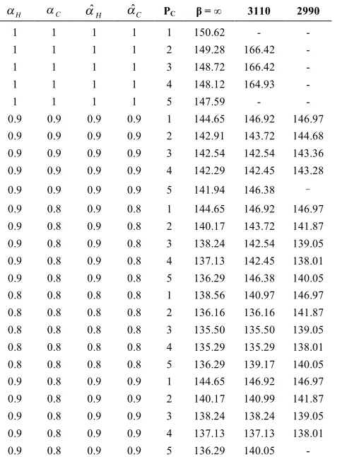
TABLE 2. Total routing cost of SA-TH-HM for IAD data with
37 nodes and PH=5
H
a aC aˆH aˆC PC β = ∞ 3110 2990
1 1 1 1 1 150.62 - -
1 1 1 1 2 149.28 166.42 -
1 1 1 1 3 148.72 166.42 -
1 1 1 1 4 148.12 164.93 -
1 1 1 1 5 147.59 - -
0.9 0.9 0.9 0.9 1 144.65 146.92 146.97
0.9 0.9 0.9 0.9 2 142.91 143.72 144.68
0.9 0.9 0.9 0.9 3 142.54 142.54 143.36
0.9 0.9 0.9 0.9 4 142.29 142.45 143.28
0.9 0.9 0.9 0.9 5 141.94 146.38
-0.9 0.8 0.9 0.8 1 144.65 146.92 146.97
0.9 0.8 0.9 0.8 2 140.17 143.72 141.87
0.9 0.8 0.9 0.8 3 138.24 142.54 139.05
0.9 0.8 0.9 0.8 4 137.13 142.45 138.01
0.9 0.8 0.9 0.8 5 136.29 146.38 140.05
0.8 0.8 0.8 0.8 1 138.56 140.97 146.97
0.8 0.8 0.8 0.8 2 136.16 136.16 141.87
0.8 0.8 0.8 0.8 3 135.50 135.50 139.05
0.8 0.8 0.8 0.8 4 135.29 135.29 138.01
0.8 0.8 0.8 0.8 5 136.29 139.17 140.05
0.9 0.8 0.9 0.9 1 144.65 146.92 146.97
0.9 0.8 0.9 0.9 2 140.17 140.99 141.87
0.9 0.8 0.9 0.9 3 138.24 138.24 139.05
0.9 0.8 0.9 0.9 4 137.13 137.13 138.01
0.9 0.8 0.9 0.9 5 136.29 140.05 -
CPU time of SA-TH-CHM and SA-TH-HM models for (aH,aC,aˆH,aˆC)=(0.9,0.8,0.9,0.8), β=∞ and PH= 5 in
different cases of PC=1,2,3,4,5 are depicted in Figure
11.
It could be seen that CPU time by increase in PC from 1 to 5 in SA-TH-CHM is exactly similar to CPU time trend for SA-TH-HM, and interestingly, these two times are similar in two states of PC = {3,5} and there is
a very small difference between three remaining times. The smallest magnitudesβ for different values of discount coefficients were calculated and 2870 was the smallest magnitude through which a justified answer for all cases could be achieved.
Then, other magnitudes with increasing trend of 120-unit were selected as well. Similar to the work by other researcher [28], we calculated the amounts of β. Therefore, we defined β∈ {2990, 3110, ∞} for the IAD
data. For an infeasible situation, we do not have any report. For each amount of outputs of the problem with different discount coefficients have been solved (see the results in Table 1 to 6.) In order to consider a larger solution space and have feasible solutions for other magnitudes of discount coefficients.
TABLE 3. Locations of central habs and hubs in the
SA-TH-CHM for IAD data with 37 nodes and PH=5
) αˆ , αˆ , α ,
(αH C H C β P
c Central hubs Hubs
(0.9, 0.9, 0.9, 0.9)
2990 3110 1 2 3 4 5 1 2 3 4 28 10,28 10,19,31 2,10,19,31 10 10,31 10,19,31 10,16,19,31 28,10,23,15,32 10,28,31,36,23 2,10,19,31,36 2,10,19,31,36 -2,31,10,35,15 2,31,10,23,15 2,10,31,19,15 10,16,31,19,15
(0.9, 0.8, 0.9, 0.8)
∞ 2990 3110 5 1 2 3 4 5 1 2 3 4 5 1 2,10,16,19,31 31 10,31 10,19,31 10,16,19,31 2,10,16,19,31 28 19,31 10,19,31 10,16,19,31 2,10,16,19,31 10 2,10,16,19,31 31,10,23,16,30 2,31,10,23,15 2,10,15,19,31 10,16,19,31,15 2,10,16,19,31 10,15,23,28,32 3,10,15,19,31 2,10,19,31,36 10,16,19,31,2 2,10,16,19,31 2,31,10,35,15
(0.8, 0.8, 0.8, 0.8)
∞ 2990 2 3 4 5 1 2 3 4 5 1 2 3 10,31 10,19,31 10,16,19,31 10,16,19,28,31 31 10,31 10,19,31 10,16,19,31 2,10,16,19,31 10 10,31 10,19,31 2,31,10,23,15 2,31,10,19,15 10,16,19,31,15 10,16,19,28,31 31,10,16,23,30 2,31,10,23,15 2,10,19,31,15 10,16,19,31,15 2,10,16,19,31 2,31,10,19,15 2,31,10,23,15 2,10,19,15,31 3110 ∞ 4 5 1 2 3 4 5 1 2 3 4 5 10,16,19,31 2,10,16,19,31 10 10,31 10,19,31 10,16,19,31 10,16,19,28,31 31 10,31 10,19,31 10,16,19,31 2,10,16,19,31 10,16,19,31,15 2,10,16,19,31 2,31,10,19,15 2,31,10,23,15 2,10,15,19,31 10,16,19,31,15 10,16,19,28,31 10,16,23,30,31 2,10,31,15,23 2,10,15,19,31 10,16,19,31,15 2,10,16,19,31
(0.9, 0.8, 0.9, 0.9) 2990
TABLE 4. Locations of central habs and hubs in the
SA-TH-HM for IAD data with 37 nodes and PH=5
) ˆ , ˆ , ,
(aHaCaHaC β Pc Central hubs Hubs
(0.9, 0.9, 0.9, 0.9)
2990 3110 1 2 3 4 5 1 2 3 4 5 10 10,31 10,19,31 10,16,19,31 -10 10,31 10,19,31 10,16,19,31 2,10,16,19,31 2,31,10,35,14 2,31,10,23,14 2,31,10,19,14 16,10,31,19,14 2,31,10,35,15 2,31,10,23,14 2,10,31,19,15 10,16,31,19,15 2,10,16,19,31
(0.9, 0.8, 0.9, 0.8)
∞ 2990 3110 1 2 3 4 5 1 2 3 4 5 1 31 10,31 10,19,31 2,10,16,31 2,10,16,19,31 10 10,31 10,19,31 10,16,19,31 2,10,16,19,31 10 31,10,23,12 2,31,10,23,15 2,10,15,19,31 2,10,16,23,31 2,10,16,19,31 2,31,10,35,14 2,31,10,23,14 2,10,19,31,15 10,16,19,31,14 2,10,16,19,31 2,31,10,35,15
(0.8, 0.8, 0.8, 0.8)
∞ 2990 2 3 4 5 1 2 3 4 5 1 2 3 10,31 10,19,31 10,16,19,31 10,16,19,28,31 31 10,31 10,19,31 10,16,19,31 2,10,16,19,31 10 10,31 10,16,31 2,31,10,23,14 2,31,10,19,15 10,16,19,31,15 10,16,19,28,31 31,10,23,12,30 2,31,10,23,15 2,10,19,31,15 10,16,19,31,15 2,10,16,19,31 2,31,10,19,15 2,31,10,23,15 16,31,10,23,15 3110 ∞ 4 5 1 2 3 4 5 1 2 3 4 5 10,16,19,31 2,10,16,19,31 10 10,31 10,16,31 10,16,19,31 10,16,19,28,31 31 10,31 10,16,31 10,16,19,31 2,10,16,19,31 10,16,19,31,15 2,10,16,19,31 2,31,10,19,15 2,31,10,23,15 10,16,31,23,15 10,16,19,31,15 10,16,19,28,31 12,10,31,23,30 2,31,10,23,15 10,15,16,23,31 10,16,19,31,15 2,10,16,19,31
(0.9, 0.8, 0.9, 0.9)
(1, 1,1,1) 2990 3110 ∞ 3110 ∞ 1 2 3 4 5 1 2 3 4 5 1 2 3 4 5 3 4 5 1 2 3 4 5 10 10,31 10,19,31 10,16,19,31 -10 10,31 10,19,31 10,16,19,31 2,10,16,19,31 31 10,31 10,19,31 10,16,19,31 2,10,16,19,31 10,28 10,28,31 10,16,28,31 31 10,31 10,16,31 2,10,16,31 2,10,16,19,31 2,31,10,35,14 2,10,14,23,31 2,10,14,19,31 10,14,16,19,31 -2,31,10,35,15 2,10,31,23,14 2,10,15,19,31 10,15,16,19,31 2,10,16,19,31 10,23,31,12 2,10,15,19,31 10,15,16,19,31 2,10,16,19,31 10,28,31,23,35 10,28,31,23,35 10,16,28,31,23 10,12,23,31 2,10,15,23,31 2,10,16,23,31 2,10,16,23,31 2,10,16,19,31
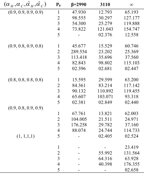
TABLE 5. Elapse times in the SA-TH-CHM for IAD data with
37 nodes and PH=5
∞ 3110 β=2990 P0 ) ˆ , ˆ , ,
(aH aC aH aC
65.193 127.177 119.888 154.747 12.558 60.746 25.369 37.560 115.103 02.447 63.200 117.142 119.455 93.318 02.440 62.003 24.971 37.160 114.733 02.524 23.419 131.564 63.928 176.355 02.658 12.793 30.297 25.279 121.043 02.376 15.529 23.202 35.696 98.802 02.681 29.599 83.214 110.892 103.071 02.849 13.821 21.511 29.782 24.744 02.405 55.992 64.316 40.398 47.930 98.555 54.300 73.822 45.677 289.554 113.418 82.843 02.396 15.595 84.361 90.132 65.607 02.381 67.761 104.005 176.258 88.074 -1 2 3 4 5 1 2 3 4 5 1 2 3 4 5 1 2 3 4 5 1 2 3 4 5 (0.9, 0.9, 0.9, 0.9)
(0.9, 0.8, 0.9, 0.8)
(0.8, 0.8, 0.8, 0.8)
(0.9, 0.8, 0.9, 0.9)
(1, 1,1,1)
TABLE 6. Elapse times in the SA-TH-HM for IAD data with
37 nodes and PH=5
∞ 3110 β=2990 P0 ) ˆ , ˆ , ,
(aH aCaH aC
39.471 47.598 92.591 90.339 01.740 35.047 12.957 41.448 82.562 01.718 12.567 66.480 92.106 75.388 01.838 35.304 13.235 42.078 85.278 01.735 11.716 115.172 124.353 115.077 01.527 47.168 100.791 98.666 85.797 01.899 37.492 79.730 87.359 83.467 02.235 53.960 43.631 82.854 74.287 02.194 63.365 91.476 80.279 82.605 01.890 -48.261 95.957 21.902 - 17.597 70.601 95.803 74.814 -34.632 55.837 61.046 53.481 01.873 66.763 57.299 75.546 79.768 01.837 17.974 48.102 67.394 49.123 - - - - - - 1 2 3 4 5 1 2 3 4 5 1 2 3 4 5 1 2 3 4 5 1 2 3 4 5
(0.9, 0.9, 0.9, 0.9)
(0.9, 0.8, 0.9, 0.8)
(0.8, 0.8, 0.8, 0.8)
(0.9, 0.8, 0.9, 0.9)
4. CONCLUDING REMARKS
The present paper attempts to develop, create and solve a new and applied model in the same trend of the previous studies on the hub location literature. The model known as a capacitated hierarchical hub median location problem is taking advantage of some significant capabilities such as the development of the previous models with imposing capacity situations in a hierarchical structure. Thus, these significant changes have occurred with the least cost in the least possible solving time of problem. These situations are confirmed that the present model is unique in its own kind. Therefore, this paper contributes to the literature on hub location problems to move towards real situations. We study a new model with title of capacitated hierarchical hub median location problem and use the real-world dataset in hub location problem corresponded to Iranian hub airport location. Results showed that the new model has changed the structure of the network and location of services facilities (i.e., hubs and central hubs). Therefore, in practice outcome network of the previous models have not been responsive the demand of applicants of services. As a result, the network structure with the capacity on the hubs facilities has been transform into a logical framework. However, since there is no end of the knowledge for the model developed in this paper, improvement situations can be considered such as multi-objective modeling with objectives of fixed charge costs of the hubs, the central hubs and linking among them or imposing multi-allocation situations along with single multi-allocation ones.
5. REFERENCES
1. O'kelly, M. E., "A quadratic integer program for the location of interacting hub facilities", European Journal of Operational Research, Vol. 32, No. 3, (1987), 393-404.
2. Campbell, J. F., "Integer programming formulations of discrete
hub location problems", European Journal of Operational
Research, Vol. 72, No. 2, (1994), 387-405.
3. Skorin-Kapov, D., Skorin-Kapov, J. and O'Kelly, M., "Tight
linear programming relaxation of uncapacitated p-hub median problems", Location Science, Vol. 5, No. 1, (1997), 68-69. 4. Ernst, A. T. and Krishnamoorthy, M., "Efficient algorithms for
the uncapacitated single allocation p-hub median problem",
Location Science, Vol. 4, No. 3, (1996), 139-154.
5. Campbell, J. F., Ernst, A. T. and Krishnamoorthy, M., "Hub
location problems", Facility Location: Applications and
Theory, Vol. 1, (2002), 373-407.
6. Alumur, S. and Kara, B. Y., "Network hub location problems:
The state of the art", European Journal of Operational
Research, Vol. 190, No. 1, (2008), 1-21.
7. Chen, H., Campbell, A. M. and Thomas, B. W., "Network
design for time‐constrained delivery", Naval Research Logistics (NRL), Vol. 55, No. 6, (2008), 493-515.
8. Labbé, M. and Yaman, H., "Solving the hub location problem in
a star–star network", Networks, Vol. 51, No. 1, (2008), 19-33. 9. Wagner, B., "Model formulations for hub covering problems",
Journal of the Operational Research Society, Vol. 59, No. 7, (2007), 932-938.
10. Yoon, M.-G. and Current, J., "The hub location and network design problem with fixed and variable arc costs: formulation and dual-based solution heuristic", Journal of the Operational Research Society, Vol. 59, No. 1, (2006), 80-89.
11. Alumur, S. and Kara, B. Y., "A hub covering network design problem for cargo applications in Turkey", Journal of the Operational Research Society, Vol. 60, No. 10, (2008), 1349-1359.
12. Alumur, S. A., Kara, B. Y. and Karasan, O. E., "The design of
single allocation incomplete hub networks", Transportation
Research Part B: Methodological, Vol. 43, No. 10, (2009), 936-951.
13. Calık, H., Alumur, S. A., Kara, B. Y. and Karasan, O. E., "A tabu-search based heuristic for the hub covering problem over incomplete hub networks", Computers & Operations Research, Vol. 36, No. 12, (2009), 3088-3096.
14. Campbell, J. F., "Hub location for time definite transportation",
Computers & Operations Research, Vol. 36, No. 12, (2009), 3107-3116.
15. Contreras, I., Fernández, E. and Marín, A., "Tight bounds from a path based formulation for the tree of hub location problem",
Computers & Operations Research, Vol. 36, No. 12, (2009), 3117-3127.
16. Ernst, A. T., Hamacher, H., Jiang, H., Krishnamoorthy, M. and Woeginger, G., "Uncapacitated single and multiple allocation p-hub center problems", Computers & Operations Research, Vol. 36, No. 7, (2009), 2230-2241.
17. Limbourg, S. and Jourquin, B., "Optimal rail-road container terminal locations on the European network", Transportation Research Part E: Logistics and Transportation Review, Vol. 45, No. 4, (2009), 551-563.
18. Meyer, T., Ernst, A. T. and Krishnamoorthy, M., "A 2-phase algorithm for solving the single allocation p-hub center problem", Computers & Operations Research, Vol. 36, No. 12, (2009), 3143-3151.
19. Sim, T., Lowe, T. J. and Thomas, B. W., "The stochastic p-hub center problem with service-level constraints", Computers & Operations Research, Vol. 36, No. 12, (2009), 3166-3177. 20. Contreras, I., Fernández, E. and Marín, A., "The tree of hubs
location problem", European Journal of Operational Research,
Vol. 202, No. 2, (2010), 390-400.
21. Lin, C.-C., "The integrated secondary route network design model in the hierarchical hub-and-spoke network for dual
express services", International Journal of Production
Economics, Vol. 123, No. 1, (2010), 20-30.
22. Meng, Q. and Wang, X., "Intermodal hub-and-spoke network design: incorporating multiple stakeholders and multi-type containers", Transportation Research Part B: Methodological, Vol. 45, No. 4, (2011), 724-742.
23. Yaman, H., "Allocation strategies in hub networks", European Journal of Operational Research, Vol. 211, No. 3, (2011), 442-451.
24. Ishfaq, R. and Sox, C. R., "Hub location–allocation in
intermodal logistic networks", European Journal of
Operational Research, Vol. 210, No. 2, (2011), 213-230. 25. Alumur, S. A., Kara, B. Y. and Karasan, O. E., "Multimodal hub
location and hub network design", Omega, Vol. 40, No. 6, (2012), 927-939.
26. Alumur, S. A., Yaman, H. and Kara, B. Y., "Hierarchical multimodal hub location problem with time-definite deliveries",
Transportation Research Part E: Logistics and Transportation Review, Vol. 48, No. 6, (2012), 1107-1120.
27. Elmastaş, S., "Hub location problem for air-ground
transportation systems with time restrictions", Bilkent University, (2006),
28. Yaman, H., "The hierarchical hub median problem with single
assignment", Transportation Research Part B: Methodological,
Vol. 43, No. 6, (2009), 643-658.
29. Aykin, T., "Lagrangian relaxation based approaches to
Journal of Operational Research, Vol. 79, No. 3, (1994), 501-523.
30. Jaillet, P., Song, G. and Yu, G., "Airline network design and hub location problems", Location Science, Vol. 4, No. 3, (1996), 195-212.
31. Ernst, A. T. and Krishnamoorthy, M., "Solution algorithms for the capacitated single allocation hub location problem", Annals of Operations Research, Vol. 86, (1999), 141-159.
32. Labbé, M., Yaman, H. and Gourdin, E., "A branch and cut algorithm for hub location problems with single assignment",
Mathematical Programming, Vol. 102, No. 2, (2005), 371-405.
33. da Graça Costa, M., Captivo, M. E. and Clímaco, J.,
"Capacitated single allocation hub location problem—A bi-criteria approach", Computers & Operations Research, Vol. 35, No. 11, (2008), 3671-3695.
34. Tavakkoli-Moghaddam, R., Gholipour-Kanani, Y. and Shahramifar, M., "Comparing three proposed meta-heuristics to solve a new p-hub location-allocation problem", International Journal of engineering, Transactions C: Aspects, Vol. 26, No. 6, (2013), 605-620.
35. Ebery, J., Krishnamoorthy, M., Ernst, A. and Boland, N., "The capacitated multiple allocation hub location problem:
Formulations and algorithms", European Journal of
Operational Research, Vol. 120, No. 3, (2000), 614-631. 36. Sasaki, M. and Fukushima, M., "On the hub-and-spoke model
with arc capacity constraints", Journal of the Operations Research Society of Japan-Keiei Kagaku, Vol. 46, No. 4, (2003), 409-428.
37. Boland, N., Krishnamoorthy, M., Ernst, A. T. and Ebery, J., "Preprocessing and cutting for multiple allocation hub location problems", European Journal of Operational Research, Vol. 155, No. 3, (2004), 638