A Multi-objective Imperialist Competitive Algorithm for a Capacitated Single-allocation Hub Location Problem

International Journal of Engineering

A Multi-objective Imperialist Competitive Algorithm for a Capacitated

Single-allocation Hub Location Problem

R. Tavakkoli-Moghaddama*_{, Y. Gholipour-Kanani}b_{, M. Shahramifar}c

a _{Department of Industrial Engineering, College of Engineering, University of Tehran, Tehran, Iran} b _{Department of Management, Qaemshahr Branch, Islamic Azad University, Qaemshahr, Iran} c _{Department of Industrial Engineering, Mazandaran University of Science & Technology, Babol, Iran}

P A P E R I N F O

Paper history:

Received 26 March 2012

Received in revised form 18 October 2012 Accepted 24 January 2013

Keywords: Hub Location Single Allocation Capacity Choice

Multi-objective Imperialist Competitive Algorithm

NSGA-II

A B S T R A C T

This paper presents a novel multi-objective mathematical model for a capacitated single-allocation hub location problem. There is a vehicle capacity constraint considered in this model. Additionally, our model balances the amount of the incoming flow to the hubs. Moreover, there is a set of available capacities for each potential hub, among which one can be chosen. The multiple objectives are to minimize the total cost of the networks regarding minimizing the maximum travel time between nodes. Due to the NP-hard property of this problem, the model is solved by a multi-objective imperialist competitive algorithm (MOICA). To prove its efficiency, the related results are compared with the results obtained by the well-known multi-objective evolutionary algorithm, namely NSGA-II. The results confirm the efficiency and the effectiveness of our proposed MOICA to provide good solutions, especially for medium and large-sized problems. Finally, we conclude that the proposed MOICA finds quality solutions rather than the solutions obtained by the NSGA-II algorithm.

doi:10.5829/idosi.ije.2013.26.06c.06

1. INTRODUCTION 1

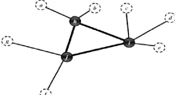
In the network design, connecting of the terminal nods by direct links can be very costly and very busy. Therefore, it is a better traffic demand from origin nodes to destination nodes through other nodes, called hubs. For example, Figure 1 depicts the structure, in which there are direct connections between of nodes, and Figure 2 shows the network with indirect connection and three hubs. Hub facilities serve as switching and transshipment used for indirect connection between terminal nods. The aim of a hub location problem is to find location of the hubs and to assign non-hub nodes (so-called spokes) to the located hubs. In hub location problems, the cost of hub-to-hub transportation is multiplied by a reduction factor of αÎ[0,1] due to consolidation of flows. A hub location problem is applied in airline postal [1], transportation [2], telecommunications network [3] postal network [4] and emergency services [5, 6].

*Corresponding Author Email: [email protected] (R. Tavakkoli-Moghaddam)

Figure 1. Fully connected network with 10 nodes and 10 origin/destination pairs

The classical objective function in a hub location problem is divided to five major classes, namely p-hub median, hub location with fixed cost, p-hub center, hub covering and hub edge location problems. In the p-hub median problem, locating p-hubs and assigning spokes to hub nodes are the main purpose of the p-hub problems in such a way that the total transportation cost is minimized. The hub net work consists of two basic types, namely single and multiple allocations. In single allocation, each non-hub node is allocated to unique hub, as shown Figure 3. Many of delivery systems are in a form of single allocation. O’Kelly [7] produced the first mathematical model for the hub location problem. He proposed a quadratic integer programming for a single allocation p-hub median problem. Campbell [5] presented the first linear integer programming formulation for the single-allocation p-hub median problem. A number of researchers have discussed single allocation hub problems [4, 8-12]. In multiple allocations, each non-hub node can be allocated to more than one hub, as shown in Figure 4. In an air network, many of origins allocate to more than one hub. Campbell [13] produced the first linear integer programming formulation for multiple allocation p-hub median problems. In addition, other researchers studied multiple allocation hub problems [14-17].

Aim of a hub location problem with the fixed cost is similar to p-hub median problem, but in this problem, the fixed cost of locating hub is considered. O’kelly [18] proposed the single allocation hub location problem with fixed cost of installation hub such that the number of hub is not fixed. Since the number of hubs is not fixed, hub location problems with fixed cost can be classified according to the capacity constraint: capacitated and incapacitated hubs.

Figure3. Single-allocation hub location problem

Figure4. Multiple-allocation hub location problem

There are different kinds of capacity constraints in hub problems; a limitation on amount of incoming flow to the hub facilities. In addition of limits on amount of flow, there is another limitation on the number of spoke nodes that can be allocated to a single hub [19]. Campbel [5] and Abdinnour-Helm and Venkataramanan [20] presented incapacitated hub location models.

In this paper, we present a bi-criteria model, whose objectives conflict each other (i.e., decreasing one criterion implies an increase in other criterion. Hub location belongs to the class of NP-hard problems. Then, we propose the imperialist competitive algorithm (ICA) and NSGA-II to solve the capacitated single allocation multiple objective hub location problem. This paper is structured as follows. Section 2 describes the research background. A brief description of the research design and the problem formulation are provided in Section 3. Section 4 proposes the imperialist competitive algorithm. The experimental results are presented in Section 5. Finally, Section 6 presents conclusion of this paper.

2. RESEARCH BACKGROUND

presented a study considered a bi-criteria model with two objectives (i.e., cost and process time of hubs), simultaneously. The first and second models minimize the entire transportation cost model and the maximum processing time in the hub, respectively.

Various heuristic methods have been proposed for solving this problem. Simulated annealing (SA) for the single allocation p-hub median problem was presented by Ernst and Krishnamoorthy [4], Abdinnour-Helm [33]. Tabu search (TS) for the single allocation p-hub median problem was developed by Skorin-Kapov and Skorin-Kapov [34], Klincewicz [35]. Ernest and Krishnamoorthy [36] presented a branch-and-bound method with the initial upper bound provided by SA and random descent heuristic methods for a capacitated single allocation p-hub location problem. A branch-and-cut algorithm based on investigations of some polyhedral properties of the capacitated single allocation hub location problem is studied by Labbe et al. [37]. Contras et al. [38] presented the heuristic method to produce Lagrangian dual feasible solutions for a capacitated single allocation hub location problem. The first heuristic method for single allocation p-hub center problem is proposed by Pumak and Sepil [39]. Ernest et al. [23] presented five heuristic algorithms for a single allocation p-hub center problem and analyzed their worst case performances. Gavriliouk [40] studied the heuristic method for single and multiple allocation p -hub centers.

As mentioned above, a variety of hub location models have been studied during the last decades. However, studies on competitive hub location problems are scarce. In a real situation, several firms usually exist in a market and compete with each other in order to capture the market share. We can easily imagine that hub locations are affected by competing with rival firms. Marianov et al. [41] formulated a competitive hub location problem on a network, which seems to be the first hub location model considering competition. In their model, the sum of captured flows is maximized under some passengers’ allocation rules. Sasaki et al. [16] considered a continuous hub location model, in which two firms of a similar size locate their own new hubs in an arbitrary order, and formulated a leader's problem as a bi-level programming problem. The numerical experiments reported in article [16] show that the leader firm may suffer heavy losses if it neglects to consider the competitors’ strategies.

Hub location problems are NP-hardness with the exception of a few special cases. They are usually much harder to solve in comparison with other non-hub location problems. Moreover, there does not exist a general mathematical model that describes well all hub location problems. Each hub problem has its own specific structure, namely objective function, decision variables and constraints. A few additional constraints or a slight modification of the problem structure can

substantially change the computational behavior of the designed solution approach. Therefore, there is no general algorithm for solving all hub problems, or at least a smaller group of them. Exact methods cannot provide solutions for large-scale hub location problems, which arise from practice in a reasonable amount of time. Therefore, heuristic methods are very promising approaches for solving hub location problems. A detailed review of hub location problems and solution methods for solving them can be found in article [41].

3. PROBLEM FORMULATION

Alumur et al. [12] presented the single allocation incomplete p-hub median, the incomplete hub location with fixed costs, the incomplete hub covering and the incomplete p-hub center problems. Our problem is an extension of the Alumur‘s model. Our model minimizes the cost and time between nodes simultaneously as the hubs are incomplete. This model balances the flow between hubs. In addition, the vehicle capacity constraint is considered. The problem is formulated according to the following assumptions:

· The hub network is not necessary complete.

· There are economies of scale incorporated by a discount factor αÎ[0,1) for using inter-hub connections

· The demand for every node is fixed.

· The cost transportation of one unit of flow between a spoke and a hub based on distance is fixed and definite.

· Each spoke allocate to only one hub(i.e., single allocation)

· Different capacity levels are available for a potential hub to be located at node k, among which one can be chosen (kÎN).

· Fixed cost of locating a hub with capacity of level q at nod k is definite. (kÎN , qÎ )

· Transportation of commodity from origin to hub

is not continuous.

· The number of vehicles is limited since there is traffic.

· The capacity of vehicle is definite.

· Vehicle capacity constraint and capacity

sensitive items. For example, if there are 50 packets in the origin node and the capacity of each vehicle is 10 packets, in this situation these packets are transported by 5 vehicles. However, if the number of packets is 55, then [

] =5 vehicles is assigned and 5 commodities are remained. In this case, there are two states. In the first state, a vehicle should be waited to complete and then move that we have more time rather than the average real time between an origin and a hub. Therefore, each commodity includes the delay cost. In the second state, a vehicle should be moved with incomplete capacity moves. Since the transportation cost of a vehicle is divided by the number of commodities, so the cost of transportation of a unit flow is heavier. However, in this instance, commodities are sent to a hub from the origin with a less time rather than the average real time. Using the extended vehicle in the hub is not applicable since hubs are more congest.

In this paper, one of assumptions refers to the balance parameter. In the instance with 8 nodes, the optimal network design is given in Figure 5. In the optimal solution, nodes 3, 4 and 5 are selected to become hubs. Nodes 1 and 7 are allocated to hub 3 (incoming 262 commodities to hub 3), nodes 2 and 8 are allocated to hub 5 (incoming 159 commodities to hub 5) and node 6 is allocated to hub 4 (incoming 189 commodities to hub 4). In this case, the difference between the maximum and the minimum amount of flows assigned to some hubs (nodes 3 and 5) is equivalent to 103. Using the balance parameter,

Figure 5. Optimal network design (instance)

Figure 6. Optimal network design with the balance parameter

the quantity of difference can be lesser. The balancing requirement is also produced in order to reduce the traffic in some hub. If the balancing parameter constraints are used, the quantity of difference should be at most equal to 46 units. In this case, the optimal solution is changed (Figure 6). Moreover, hubs 4 and 5 now operates with their second capacity level in respect to 250 and 300, respectively.

3. 1. Notations

3. 1. 1. Subscripts

N= {1,…,n} Set of nodes.

H= {1,…,h} Set of potential hub ( Î ). Qk = {1,…,sk} Set of the difference capacity levels

available for the potential hub to be installed at node k, where kÎ H.

3. 1. 2. Input Parameters

Total flow to be sent from node i to node j (i,jÎ N).

Average time of sending the flow from node i

to node j (i,jÎN).

Cost for sending one unit of the flow from node i to node j (i,jÎN).

Capacity for each vehicle

At most number of the extension vehicle in a path origin-hub

Delay cost for one unit of the remaining flow at

each hour

Fixed cost for installing a hub with capacity level q at node K (kÎH, qÎ ).

Fixed cost for installing a hub link i-j (i,jÎH). Γ Capacity of a hub installed at node k with a

level of capacity q (kÎH, qÎ ).

α Constant cost discount factor for travel on the

inter-hub connections.

′ Constant time discount factor for travel on the

inter-hub connections.

Maximum value allowed for the difference between the maximum and the minimum amount of flows assigned to the some hubs.

3. 1. 3. Decision Variables

Time for sending the flow from node i to node

k (iÎN, kÎH).

, Cost for sending the total flow originating at node i to hub k.

Amount of flows with origin at k that goes through hubs i and j (kÎN, i, jÎH).

b Upper limit on the maximum of the flow are allocated to some hubs.

Time of transportation between hubs i and j (i, jÎH).

1 if node i is assigned to hub j; 0, otherwise (iÎN, jÎH);

1 if origin i uses of an extension vehicle; 0, otherwise (iÎN).

1 if a link hub is established between hubs i and j; 0, otherwise (i,jÎH).

1 if node k receives a hub with capacity level q; 0, otherwise (kÎH,qÎ ).

1 if a spanning tree rooted at hub k using of links i and j; 0, otherwise (i,j,kÎH).

3. 2. Mathematical Model

min∑ ∑ ( , + ∑ ) +

∑ ∑ , ∑ +∑ ∑ +

∑ ∑ ;

(1)

min max _{1 + ′ + 2 ,} (2)

s.t.

, = (

∑ _{+ 1)}

+ ( ∑ +

( ∑

∑

∑ ) (∑ [

∑ _{] ))}

(1-) ∑ ≠

(3)

, =∑ ∑ = (4)

= ∑

( ∑ ) + ( ∑

∑ ∑ )

(1− ) ∑ ≠

(5)

= ∑ = (6)

≤1− " i (7)

∑ ≤ (8)

1 ≥ " , i (9)

2 ≥ " , i (10)

∑ = 1" (11)

≤ " , (12)

≤ ", : < (13)

≤ ", : < (14)

∑ : −∑ : =∑ − ∑ " ,

(15)

+ ≤ ∑ ", : < , (16)

∑ : ≥ + −1" , : ≠ (17)

∑ : ≤ " , : ≠ (18)

+ ≤ ", , : < (19)

≥( + ) ", , : ≠ , ≠ (20)

= ", : ≠ (21)

= 0" (22)

∑ ∑ ≤∑ "k (23)

∑ ≤1"k (24)

∑ ∑ + (1− )≥ "k (25)

∑ ∑ − (1− )≤ "k (26)

− ≤ (27)

, ≥ (28)

{0,1}"i , (29)

{0,1}"i (30)

≥0", (31)

{0,1}", , : ≠ , ≠ (32)

{0,1}"i,j : < (33)

{0,1}" q _, (34)

≥0"i,j : ≠ ,k (35)

Constraint (4) calculates the transportation cost of the total flow originating at origin i while the total flow originating at node i is equal to the coefficient of capacity of vehicle.

The first term of Constraint (5) is stated such that the extension vehicle is used from origin i to hub k, variable

is equal to

∑

∑ . In this case, the range of coefficient of variable is (0,1). It means that the travel time based on the amount of the flow from the origin to the hub is multiplied by a producer coefficient. Therefore, the flow is destination earlier from an average real time. The second term of Constraint (5) calculates the variable when we do not apply the extension vehicle. In this case, variable is equal to

∑ ∑

∑ + 1 . In this paper, the range

of the coefficient of variable is (1, 2). The term means that the major of the amount flow is transported by an integer number of vehicles. The remaining segment, which is lesser than the vehicle capacity, includes the delay time and the travel time based on amount of flow from the origin to the hub which is multiplied by a multiplier coefficient and therefore destination posterior from the average real time.

Constraint (6) computes the travel time from an origin to a hub, while the total flow originating at node i is equal to a multiple vehicle capacity. Constraint (7) states that the hub node is not applied more vehicles. Constraint (8) states that the number of the extended vehicle should be at most equal to a parameter since there is a limitation of traffic in the path. Constraints (9) and (10) states that a radius of a hub is greater than or equal to the collection and distribution time of going to any node allocated to this hub and the radius of spoke can be very small (i.e., close to zero), respectively. Constraint (11) assures that each spoke is allocated to exactly one hub. Constraint (12) states that a spoke can be only allocated to a hub node. Constraint (13) and (14) assure that a hub link i, j can be only established such that nodes i and j are hub nodes. Constraint (15) is the balance equation for the flow. The term on the left-hand side of the constraint calculates the flow within the hub network and the term on the right-hand side and calculates the flows allocated to the hub. In fact, the total entering flow originating from node k to hub i should be equal to the outgoing flow.

Constraint (16) states that variable to be positive if only hub link i, j is established. Constraint (17) states that the degree for each hub is at least one, and the tree rooted at hub k has an entering arc into every other hub j. Constraint (18) ensures that spanning tree rooted can be only associated with a hub and assures that each spanning tree rooted at hub k can enter at most one arc

to another hub node j. The spanning tree arcs to be hub arcs stated by Constraint (19). Constraint (20) displays that the time needed to travel between hubs is calculated by the established spanning tree rooted in the hub network. Constraint (21) states that travel time inter-hub is symmetric. Constraint (22) states that travel time from a node to itself will be zero. Constraint (23) is the capacity constraints of the hub. Constraint (24) assures that for each hub one size is chosen. Constraints (25) and (26) state that the lower and upper limits on the minimum and maximum amount of the flow are allocated to some hubs, respectively. Constraint (27) states that the difference between the maximum and minimum amounts of the flow allocated to some hubs should be at most equal to parameter θ.

4. IMPERIALIST COMPETITIVE ALGORITHM

The imperialist competitive algorithm (ICA) is a new algorithm in evolutionary computation. It is inspired by a socio-political process of imperialistic competition in the real world. This algorithm starts with an initial random population, named countries. Some of the best countries (i.e., with the least cost) are chosen to be the ‘imperialists’ and the rest are the ‘colonies’ of these imperialists. All of the colonies of the initial population are divided among the imperialists based on their power. The power of an empire is equivalent to the objective function of the proposed model.

After distribution of all colonies among imperialists, these colonies belong to their relevant imperialist country. The total power of an empire is affected by both the power of the imperialist country as a central core and the power of its colonies. Therefore, we define the total power of an empire by the sum of the power of the imperialist country and a percentage of the mean power of its colonies to their imperialists. Then, imperialistic competition begins among all the empires. Any empire, which cannot succeed and increase its power in this competition, is eliminated from the competition. Therefore, in the imperialistic competition process, the powerful empires gradually increase their power and weaker empires lose their power, and ultimately they collapse. Then, all of the empires are collapsed and there is only one empire and all the other countries are colonies of the maintained empire. Following, we explain the steps of the proposed ICA.

example, suppose we have 5 nodes and 2 capacity levels, as shown below.

1 2 1 2 2 2 1 2 1 1

Nodes 1 and 2 are hubs. The second and first capacity levels are chosen for hubs 1 and 2, respectively. In addition, nodes 3, 4 and 5 are allocated to hubs1, 2 and 2, respectively. The second matrix (n×n) consists of binary cells. It shows that the installation hub links. In addition, the third matrix (1×n) with a binary cell shows which spoke uses more vehicles.

4. 2. Initial Population Initially, any solution is made by the designed procedure, so called construct. Then the improvement procedure, so called parallel neighborhood search method, is applied for this solution to create the initial population. If the product solution is not repeated, then it is added to the population. The construction procedure and parallel neighborhood search method are explained below.

4. 2. 1. Construction Procedure Step 0- Continue until all of the nodes is considered.

Step 1- One of the nodes, which is not considered until now, is chosen as a hub at random.

Step 1-1- One of the capacity levels is chosen for hub at random.

Step 1-2- Indices, which are not considered until now, are chosen from the remaining nodes randomly. They are allocated to the located hub based on the capacity of the mentioned hub while the zero index is not produced. In addition, the second row is quantified according to the definite capacity level for the hub.

Step 2- If all of the nodes are considered, then go to the latter step; otherwise, go to the first step.

Step 3- Randomly, select 0 or 1 for each node i and j that are hubs in the second matrix, and instead on the relevant element.

Step 4- Randomly; select 0 or 1 for the element of non-hub nodes in the third matrix. Feasibility qualification for the values for matrix ( ) should be considered.

Step 5- Finish.

4. 2. 2. Parallel Neighborhood Search Procedure

This procedure consists of four neighborhood search operations, which are applied for the input solution in simultaneity or parallel. Then, one solution is selected from the input solution and solutions of these four operations on the selected solution. The first neighborhood search operation is applied for the first matrix. Randomly, two hubs is selected and one of the non-hub nodes allocated to located hubs (according to

the feasibility qualification similar to the capacity limitation) is chosen and exchanged. The second neighborhood search operation is applied for the second matrix. Randomly, two indices are chosen from the hub nodes. If the value of the relevant element is 1, then it is transmuted to 0 or if it is equaled to 0, it is transmuted to 1. In addition, the third neighborhood search operation is applied for the first matrix. Randomly, the index of one of the hub nodes is selected and its capacity level is changed to one of the available levels in according to the capacity limitation. The quarter neighborhood search operation is applied for the third matrix. Randomly, one of the non-hub nodes is chosen and if the value of this element is equaled to 1, it is changed to 0 or if it is equaled to 0, it is transmuted to 1. The general structure of this procedure is as follows: the size of population=N, input solution=s, first

operation=ls1, second operation=ls2, third

operation=ls3 and quarter operation=ls4. Step 0- Quantify 0 to the counter. Step 1- Apply ls1 for s, and obtain s1.

Step 2- Apply the improvement method (parallel neighborhood search procedure) for s1. Step 3- Apply ls2 for s, and obtain s2.

Step 4- Apply the improvement method for s2. Step 5- Apply ls3 for s, and obtain s3.

Step 6- Apply the improvement method for s3. Step 7- Apply ls4 for s, and obtain s4.

Step 8- Apply the improvement method for s4. Step 9- Choose one solution from the s, s1, s2, s3

and instead on s.

Step 10- Add one unit to the counter. If the counter is lower than the most of the definite repetition, then go to Step 1; otherwise, go to Step7.

Step 11- Report solution s as an output and finish the procedure.

4. 3. Selection Method We select one solution from the input solution and four solutions from the

produced solution according to the parallel

neighborhood search procedure. In this selection method, non-dominate relation is initially applied for five solutions and we select a solution that is not dominated by other solution. When some solutions are not dominated by other, we select solutions with the maximum distance from the dynamic idealistic point.

4. 5. Improvement Method Applying the parallel neighborhood search procedure for a solution is may be the infeasible produced solution. Therefore, an improvement method is designed in this work that applies for the produced solution. It transmutes an infeasible solution to a feasible solution. The second and third structures produce feasible solution in the respective capacity; however, the constraints related to quantity of commodity may be defected. Therefore, the improvement method updates the solutions according to two constraints of the model (i.e., Constraint 15 and 16). The solutions produced by the quarter structure may be defected by Constraint (8). So improvement methods apply for the quarter matrix and produce a feasible solution.

4. 6. Evaluation Function In this paper, these solutions are classified in to the non-dominated fronts and the crowing distance is measured for each solution relevant to its rank. Following, evaluation function( ) is calculated for every solution [41]:

= (36)

The evolution function Cs is computed for each solution,

and then the solutions are sorted in the descending order based on Cs. of the most powerful countries (i.e.,

with the minimum cost) are selected to be imperialists. The remaining countries are colonies ( ) that are allocated to an emperor based on their powers. To distribute the colonies among imperialists, the normalized cost for each emperor is computed by:

= − (37)

where, and are the normalized cost for the nth emperor and the cost of the nth emperor, respectively. Then, the proportional power of each imperialist is calculated below, and based on that the colonies are allocated to the imperialist countries.

=

∑ (38)

On one side, the normalized power of an imperialist is assessed by its colonies. Thus, the initial number of colonies of an empire is computed by:

× = { × ( )} (39)

where, × and are the initial number of

colonies of the nth empire and the number of all colonies, respectively. After that, to distribute the colonies among imperialist, × of the colonies are chosen randomly and allocated to their imperialist.

4. 7. Assimilation Methods Imperialist countries absorb the colonies countries toward themselves based on the absorption policy. In this problem, half of the hubs of the emperor are chosen randomly and located

instead of the same number of hubs with the same capacity level in each colony and the remaining nodes are allocated to the located hubs according to their capacity limitations.

4. 8. Revolution Policy One of the colonies of every emperor is chosen randomly and given to the parallel neighborhood search procedure as an input. Then, the output is instead of the colony.

4. 9. Calculation of the Cost of Imperialism The total power of an empire is affected by the power of its both parts (i.e., the emperor power and percents of its average colonies power). Therefore, the mathematical equation of the total cost is computed by:

× = (emperor ) + × {

(_{Colonies of emperor )}} (40)

where, T × C is the total cost of the nth imperialism? In addition, is a positive factor considered between 0 and 1. According to the upper relation, a little value for causes the cost of the nth imperialism closes to the cost of the nth emperor. In this paper, we consider is 0.3.

4. 10. Imperialistic Competition After computing the cost of empire, one (or some) of the weakest colonies is chosen from the weakest empires. Then, competition is made among all empires to possess this (or these) colony (or colonies). Based on the total power of empire during this competition, the most powerful empires are more likely to possess the mentioned colonies. Therefore, the weakest empire collapses in the imperialistic competition when it loses all of its colonies and their colonies are seized with a stronger imperialism. This process is continued until just one empire exists in the world.

4. 11. Comparison Metrics There are various metrics for evaluation of quality and diversity of the multi-objective evolutionary algorithm. In this paper, three metrics is considered as follows.

a. Quality Metric:This metric is used for comparison

of the quality of the Pareto solutions obtained by any method. According to this metric, all of the Pareto solutions obtained by each method are ranking. The superior percent shows that the quality of this algorithm is better. Then, the percent solutions of any method in the first rank are definite.

b. Spacing Metric: This metric tests a uniform

distribution of the obtained Pareto solutions in a solution front. This metric is defined by:

=∑ | |

c. Diversity Metrics: This metrics specifies the measure of non-dominated solution on the optimal front. The diversity metrics is computed by:

= ∑ − (42)

5. EXPERIMENTAL RESULTS

In this section, the effectiveness of the proposed ICA is compared with the non-dominated sorting genetic algorithm (NSGA-II). These algorithms are run on machine Intel Core i5-540M processor with 2.53 GHz and 4 GB of RAM.

5. 1. Test Data There are capacity levels for each potential hub in the case of the CSAMOHLP. The AP (Australian Post) data set introduced by Ernst and Krishnamoorthy [36]. Accordingly, instances with 10, 15, 20 and 25 nodes are considered. The number of capacity levels available for each hub is considered as 2, 3 and 4. The largest capacity is equal to the capacity of the AP data set instances. Then, each capacity level is equal to 70% of the capacity of the upper level (∀ ∈

Г =Г and Г = 0.7 ×Г , = 1, . . , −1 ), recursively. We consider two types of the capacity of the AP data set, namely tight and loose. We took the fixed costs of opening each hub fhk= 100. The fixed costs of establishing hub links between the nodes of the network are calculated by:

= _,{ ⁄_{⁄ }×} ∀ , ≠ (43)

where, dij is the distance between nodes i and j, and wij

is the flow between nodes i and j. For the AP data, we assumed that H=N in all at the instances.

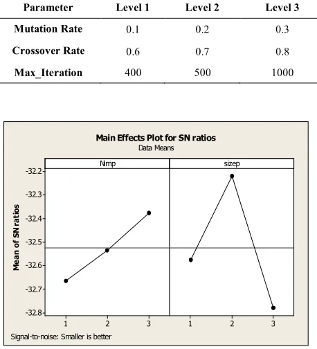
5. 2. Parameters Tuning for ICA and NSGA-II The parameters of the ICA algorithm are the number of imperialists (i.e., Imp-Num) and the number of population (i.e., Popsize). The considered levels of the parameters are shown in Table 1. In addition, the NSGA-II algorithm has three parameters, namely mutation rate, crossover rate and maximum iteration, whose levels are shown in Table 2. The associated results are analyzed by the Taguchi design method in design of experiments (DOE) and implemented in MINITAB 16. The analysis of the ICA algorithm for the levels Imp-size and Pop-size factors are shown in Figure 7. In this figure, it can be seen that the Imp-Num=10 and Pop-size=120 results in a better output in comparison with the other values in the ICA algorithm. Furthermore, the analysis of the NSGA-II algorithm for the levels of the mutation rate, crossover rate and Max-Iteration factors are shown in Figure 8. The

Imp-Num=10 and Pop-size=120 give a better output in comparison with the other values used in the ICA algorithm based on Figure 7. In addition, we set the parameters for the NSGA-II according to Figure 8. These parameters are the mutation rate=0.2, crossover rate=0.7 and max_iteration=400.

TABLE 1. Considered levels of the ICA parameters

Parameter Level 1 Level 2 Level 3

Imp-Num 10 14 16

Pop-size 70 100 120

TABLE 2. Considered levels of the NSGA-II parameters

Parameter Level 1 Level 2 Level 3

Mutation Rate 0.1 0.2 0.3

Crossover Rate 0.6 0.7 0.8

Max_Iteration 400 500 1000

3 2 1 -32.2

-32.3

-32.4

-32.5

-32.6

-32.7

-32.8

3 2 1 Nimp

M

e

a

n

o

f

S

N

r

a

ti

o

s

sizep Main Effects Plot for SN ratios

Data Means

Signal-to-noise: Smaller is better

Figure 7. Analysis of the ICA algorithm for the levels of imp-size and pop-imp-size factors

3 2 1 -51.00 -51.25 -51.50 -51.75 -52.00

3 2 1

3 2 1 -51.00 -51.25 -51.50 -51.75 -52.00

mutation rate

M

e

a

n

o

f

S

N

r

a

ti

o

s

crossover rate

max_iteration

Main Effects Plot for SN ratios

Data Means

Signal-to-noise: Smaller is better

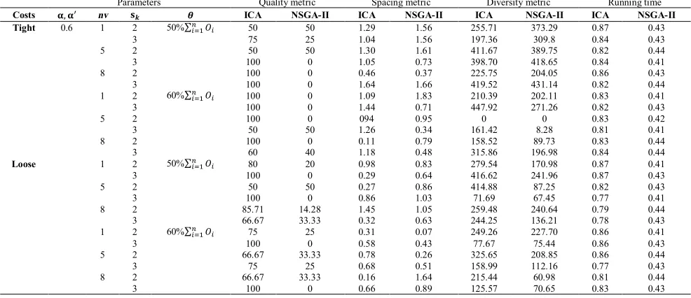
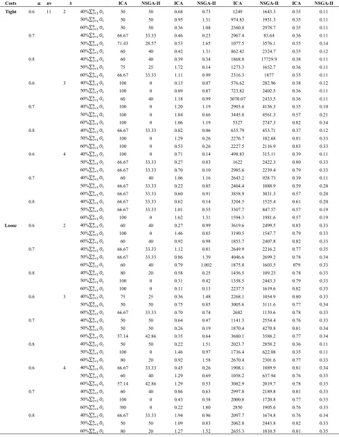
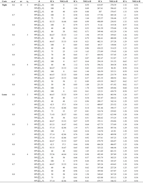
5. 3. Experimental Results In this section, the effectiveness of the proposed ICA is compared with the NSGA-II algorithm for small-sized instances. There are variant metrics for comparison between the algorithms. In this paper, these algorithms are compared based on four metrics, namely quality, spacing, diversity and running time. The results of the comparison with deferent values of parameters are illustrated in Tables 3

to 6. For each instance, the first five columns are the input parameters of the problem. The sixth column is the comparison between two algorithms based on the quality metric. The seventh column is the comparison based on the spacing metric. The eighth column shows the comparison based on the diversity metrics, and the ninth column shows the comparison based on the running time analysis.

TABLE 3. Computational comparison of the proposed ICA and the NSGA-II algorithm for n=10

Running time Diversity metric Spacing metric Quality metric Parameters NSGA-II ICA NSGA-II ICA NSGA-II ICA NSGA-II ICA nv , ′ Costs 0.25 0.46 509.13 593.13 1.76 1.44 40 60 50%∑ 2 1 0.6 Tight 0.24 0.48 233.69 691.02 0.12 1.041 0 100 3 0.25 0.45 294.94 114.26 0.82 0.61 0 100 2 2 0.24 0.47 351.83 320.91 0.95 0.94 50 50 3 0.23 0.49 152.19 411.09 0.89 0.97 40 60 2 5 0.23 0.45 265.29 69.68 0.82 0.61 0 100 3 0.24 0.46 446.86 414.08 0.94 1.51 0 100 60%∑ 2 1 0.24 0.46 346.83 607.79 0.81 0.46 33.33 66.67 3 0.24 0.46 482.16 211.99 1.06 0.05 0 100 2 2 0.23 0.46 532.94 42712 1.76 0.51 50 50 3 0.25 0.45 436.54 287.61 1.43 0.89 50 50 2 5 0.24 0.44 197.85 300.82 0.96 0.6 33.33 66.67 3 0.24 0.45 88.05 224.24 1.02 0.46 20 80 50%∑ 2 1 Loose 0.24 0.45 272.52 541.56 0.59 0.2 33.33 66.67 3 0.25 0.47 171.76 182.82 0.04 0.87 50 50 2 2 0.05 0.13 307.92 313.09 0.44 0.38 50 50 3 0.23 0.45 257.94 265.63 1.08 1.54 25 75 2 5 0.24 0.44 321.19 121.89 0.21 0.22 33.33 66.67 3 0.23 0.47 502.33 340.69 1.17 0.85 0 100 60%∑ 2 1 0.23 0.46 482.89 511.97 1.31 1.48 25 75 3 0.24 0.47 138.59 300.5 0.14 1.32 50 50 2 2 0.24 0.47 469.84 544.25 0.21 0.22 42.86 57.14 3 0.24 0.46 127.56 88.03 0.14 0.45 33.33 66.67 2 5 0.25 0.45 84.64 128.11 0.15 0.14 33.33 66.67 3

TABLE 4. Computational comparison of the proposed ICA and the NSGA-II algorithm for n=15

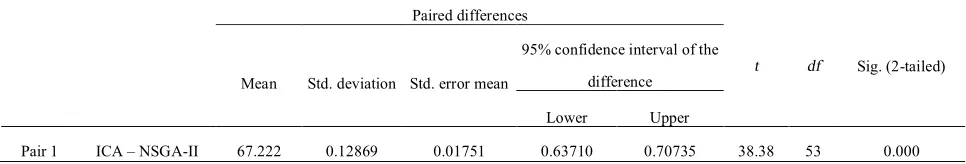
The proposed ICA and the NSGA-II algorithm for n=10 A paired t-test is conducted to see whether the significant difference exists between the obtained solution of the proposed ICA and the optimal solution of the NSGA-II algorithm. The difference between the computed values of two methods for test problem i is shown by the variable Di. Therefore, the statistics are as follows:

=√ × ; where =∑ and = ∑( ) (44)

A paired t-test is conducted by 54 test problems in the SPSS software. In these Tables 8 and 9, it can be seen that, there is not statistical significant difference between solutions obtained by ICA and NSGA-II based on spacing Metrics and diversity Metrics according to the significance (2-tailed)>0.05. However, there is statistical significant difference based on quality metrics and time metrics according to the significance (2-tailed)<0.05 in Tables 7 and 10.

TABLE 7. Detailed statistics of the paired t-test for the quality metric

TABLE 8. Detailed statistics of the paired t-test for the spacing metric

TABLE 9. Detailed statistics of the paired t-test for the diversity metric

TABLE 10. Detailed statistics of the paired t-test for the running time analysis

Paired differences

t df Sig. (2-tailed) Mean Std. deviation Std. error mean

95% confidence interval of the

difference

Lower Upper

Pair 1 ICA – NSGA-II 42.50796 34.42031 4.68401 33.11303 51.90290 9.075 53 0.000

Paired differences

t df Sig. (2-tailed) Mean Std. deviation Std. error mean

95% confidence interval of the

difference

Lower Upper

Pair 1 ICA – NSGA-II -1.86315 13.38053 1.82086 -5.51533 1.78903 -1.023 53 0.311

Paired differences

t df Sig. (2-tailed) Mean Std. deviation Std. error mean

95% confidence interval of the

difference

Lower Upper

Pair 1 ICA – NSGA-II -52.0385 297.53524 40.48942 -133.25000 29.17297 -1.285 53 0.204

Paired differences

t df Sig. (2-tailed) Mean Std. deviation Std. error mean

95% confidence interval of the

difference

Lower Upper

6. CONCLUSION

In this paper, we have studied different conflicting objectives for the capacitated single-allocation hub location problem, in which the flow has been transported non-contiguous. We have proposed two

alternative bi-objectives minimizing the total

transportation cost and minimizing the maximum travel time between all origin–destination pairs. In addition, the considered model has avoided from congestion in the hubs. We have proposed a new imperialist competitive algorithm (ICA) to solve the given problems. The performance of the proposed ICA has been compared with the NSGA-II algorithm based on the quality metric, spacing metric, diversity metric and running time analysis. The related results have been illustrated. According to the statistical analysis, the quality metric computed for the proposed ICA has been better than NSGA-II. However, the proposed ICA has needed more time to solve the problems. Furthermore, there has not been statistically significant difference between the solutions obtained by the proposed ICA and the NSGA-II algorithm based on the spacing and diversity metrics.

7. REFERENCES

1. Aykin, T., "Networking policies for hub-and-spoke systems with application to the air transportation system", Transportation Science, Vol. 29, No. 3, (1995), 201-221.

2. Aversa, R., Botter, R., Haralambides, H. and Yoshizaki, H., "A mixed integer programming model on the location of a hub port in the east coast of south america", Maritime Economics & Logistics, Vol. 7, No. 1, (2005), 1-18.

3. Chung, S.-h., Myung, Y.-s. and Tcha, D.-w., "Optimal design of a distributed network with a two-level hierarchical structure",

European Journal of Operational Research, Vol. 62, No. 1, (1992), 105-115.

4. Ernst, A. T. and Krishnamoorthy, M., "Efficient algorithms for the uncapacitated single allocation p-hub median problem",

Location Science, Vol. 4, No. 3, (1996), 139-154.

5. Campbell, J. F., "Integer programming formulations of discrete hub location problems", European Journal of Operational Research, Vol. 72, No. 2, (1994), 387-405.

6. Hakimi, S. L., "Optimum locations of switching centers and the absolute centers and medians of a graph", Operations Research, Vol. 12, No. 3, (1964), 450-459.

7. O'kelly, M. E., "A quadratic integer program for the location of interacting hub facilities", European Journal of Operational Research, Vol. 32, No. 3, (1987), 393-404.

8. Skorin-Kapov, D., Skorin-Kapov, J. and O’Kelly, M., "Tight linear programming relaxations of incapacitated p-hub median problems", European Journal of Operational Research, Vol. 94, (1996), 582-593.

9. O'Kelly, M. E., Bryan, D., Skorin-Kapov, D. and Skorin-Kapov, J., "Hub network design with single and multiple allocation: A computational study", Location Science, Vol. 4, No. 3, (1996), 125-138.

10. Sohn, J. and Park, S., "Efficient solution procedure and reduced size formulations for p-hub location problems", European Journal of Operational Research, Vol. 108, No. 1, (1998), 118-126.

11. Ebery, J., "Solving large single allocation p-hub problems with two or three hubs", European Journal of Operational Research, Vol. 128, No. 2, (2001), 447-458.

12. Alumur, S. A., Kara, B. Y. and Karasan, O. E., "The design of single allocation incomplete hub networks", Transportation Research Part B: Methodological, Vol. 43, No. 10, (2009), 936-951.

13. Campbell, J. F., "Location and allocation for distribution systems with transshipments and transportion economies of scale", Annals of Operations Research, Vol. 40, No. 1, (1992), 77-99.

14. Skorin-Kapov, D., Skorin-Kapov, J., O’kelly M. E., "Tight linear programming relaxations of incapacitated p-hub median problems", European Journal of Operational Research, Vol. 94, (1996), 582-593.

15. Ernst, A. T. and Krishnamoorthy, M., "Exact and heuristic algorithms for the incapacitated multiple allocation p-hub median problem", European Journal of Operational Research, Vol. 104, (1998), 100-112.

16. Sasaki, M., Suzuki, A. and Drezner, Z., "On the selection of hub airports for an airline hub-and-spoke system", Computers & Operations Research, Vol. 26, No. 14, (1999), 1411-1422. 17. Boland, N., Krishnamoorthy, M., Ernst, A. T. and Ebery, J.,

"Preprocessing and cutting for multiple allocation hub location problems", European Journal of Operational Research, Vol. 155, No. 3, (2004), 638-653.

18. O'Kelly, M. E., "Hub facility location with fixed costs", Papers in Regional Science, Vol. 71, No. 3, (1992), 293-306. 19. Klincewicz, J. G., "Hub location in backbone/tributary network

design: A review", Location Science, Vol. 6, No. 1, (1998), 307-335.

20. Abdinnour-Helm, S. and Venkataramanan, M., "Solution approaches to hub location problems", Annals of Operations Research, Vol. 78, (1998), 31-50.

21. Kara, B. Y. and Tansel, B. C., "On the single-assignment p-hub center problem", European Journal of Operational Research, Vol. 125, No. 3, (2000), 648-655.

22. Baumgartner, S., "Polyhedral analysis of hub center problems", Diploma Thesis, University Kaiserslautern, Germany, (2003). 23. Ernst, A. T., Hamacher, H., Jiang, H., Krishnamoorthy, M. and

Woeginger, G., "Uncapacitated single and multiple allocation p-hub center problems", Computers & Operations Research, Vol. 36, No. 7, (2009), 2230-2241.

24. Sim, T., Lowe, T. J. and Thomas, B. W., "The stochastic p-hub center problem with service-level constraints", Computers & Operations Research, Vol. 36, No. 12, (2009), 3166-3177. 25. Wagner, B., "Model formulations for hub covering problems",

Journal of the Operational Research Society, Vol. 59, No. 7, (2007), 932-938.

26. Qu, B. and Weng, K., "Path relinking approach for multiple allocation hub maximal covering problem", Computers & Mathematics with Applications, Vol. 57, No. 11, (2009), 1890-1894.

27. Nickel, S., Schobel, A. and Sonneborn, T., "Hub location problems in urban traffic networks", Mathematical Methods on Optimization in Transportation Systems, Kluwer Academic Publishers, Dordrecht, The Netherlands, (2001), 95-107. 28. Podnar, H., Skorin-Kapov, J. and Skorin-Kapov, D., "Network

European Journal of Operational Research, Vol. 137, No. 2, (2002), 371-386.

29. Campbell, J. F., Ernst, A. and Krishnamoorthy, M., "Hub arc location problems: Part i-introduction and results", Management Science, Vol. 51, No. 10, (2005), 1540-1555.

30. Yoon, M.-G. and Current, J., "The hub location and network design problem with fixed and variable arc costs: Formulation and dual-based solution heuristic", Journal of the Operational Research Society, Vol. 59, No. 1, (2006), 80-89.

31. Calık, H., Alumur, S. A., Kara, B. Y. and Karasan, O. E., "A tabu-search based heuristic for the hub covering problem over incomplete hub networks", Computers & Operations Research, Vol. 36, No. 12, (2009), 3088-3096.

32. da Graca Costa, M., Captivo, M. E. and Climaco, J., "Capacitated single allocation hub location problem—a bi-criteria approach", Computers & Operations Research, Vol. 35, No. 11, (2008), 3671-3695.

33. Abdinnour-Helm, S., "Using simulated annealing to solve the p-hub median problem", International Journal of Physical Distribution & Logistics Management, Vol. 31, No. 3, (2001), 203-220.

34. Skorin-Kapov, D. and Skorin-Kapov, J., "On tabu search for the location of interacting hub facilities", European Journal of Operational Research, Vol. 73, No. 3, (1994), 502-509.

35. Klincewicz, J. G., "Avoiding local optima in thep-hub location problem using tabu search and grasp", Annals of Operations Research, Vol. 40, No. 1, (1992), 283-302.

36. Ernst, A. T. and Krishnamoorthy, M., "Solution algorithms for the capacitated single allocation hub location problem", Annals of Operations Research, Vol. 86, (1999), 141-159.

37. Labbe, M., Yaman, H. and Gourdin, E., "A branch and cut algorithm for hub location problems with single assignment",

Mathematical Programming, Vol. 102, No. 2, (2005), 371-405. 38. Contreras, I., Fernandez, E. and Marin, A., "Tight bounds from a path based formulation for the tree of hub location problem",

Computers & Operations Research, Vol. 36, No. 12, (2009), 3117-3127.

39. Pamuk, F. S. and Sepil, C., "A solution to the hub center problem via a single-relocation algorithm with tabu search", IIE Transactions, Vol. 33, No. 5, (2001), 399-411.

40. Gavriliouk, E. O., "Aggregation in hub location problems",

Computers & Operations Research, Vol. 36, No. 12, (2009), 3136-3142.

A Multi-objective Imperialist Competitive Algorithm for a Capacitated

Single-allocation Hub Location Problem

R. Tavakkoli-Moghaddama_{, Y. Gholipour-Kanani}b_{, M. Shahramifar}c

a _{Department of Industrial Engineering, College of Engineering, University of Tehran, Tehran, Iran} b _{Department of Management, Qaemshahr Branch, Islamic Azad University, Qaemshahr, Iran} c _{Department of Industrial Engineering, Mazandaran University of Science & Technology, Babol, Iran}

P A P E R I N F O

Paper history:

Received 26 March 2012

Received in revised form 18 October 2012 Accepted 24 January 2013

Keywords: Hub Location Single Allocation Capacity Choice

Multi-objective Imperialist Competitive Algorithm

NSGA-II

هﺪﯿﮑﭼ

ﻪﺋارابﺎﻫ ﯽﺑﺎﯾنﺎﮑﻣ ياﺮﺑﺖﯿﻓﺮﻇ ﺖﯾدوﺪﺤﻣ وﯽﮑﺗﺺﯿﺼﺨﺗ ﺎﺑ ﻪﻓﺪﻫﺪﻨﭼ ﺪﯾﺪﺟلﺪﻣ ﮏﯾ،ﻪﻟﺎﻘﻣ ﻦﯾارد

ﯽﻣ ددﺮﮔ .

بﺎﻫﻪﺑهﺪﺷدراويﺎﻫﻻﺎﮐراﺪﻘﻣﺖﯾدوﺪﺤﻣوﻪﯿﻠﻘﻧﻞﯾﺎﺳوﺖﯾدوﺪﺤﻣ

ردنﺎﯾﺮﺟراﺪﻘﻣزﺎﯿﻧدرﻮﻣلدﺎﻌﺗﻦﺘﻓﺮﮔﺮﻈﻧردﺎﺑﺎﻫ

بﺎﻫﻦﯿﺑ

،ﺎﻫ

ﯽﻣﻪﺘﻓﺮﮔﺮﻈﻧرد

دﻮﺷ .

دﻮﺟﻮﻣحﻮﻄﺳزاﯽﮑﯾﺎﻬﻨﺗﻪﮐﺖﺳادﻮﺟﻮﻣﺖﯿﻓﺮﻇﻦﯾﺪﻨﭼبﺎﻫﺮﻫياﺮﺑ،هوﻼﻋﻪﺑ

بﺎﻫزاﮏﯾﺮﻫياﺮﺑ

ﯽﻣبﺎﺨﺘﻧاﺎﻫ

دﻮﺷ .

ﺮﺜﮐاﺪﺣندﺮﮐﻞﻗاﺪﺣﻪﺑﻪﺟﻮﺗﺎﺑارﻪﮑﺒﺷردﻞﻤﺣﻪﻨﯾﺰﻫﻞﮐ،ﻪﻓﺪﻫﺪﻨﭼلﺪﻣﻦﯾا

ﯽﻣﻞﻗاﺪﺣ،ﻪﮑﺒﺷردﻞﯾﻮﺤﺗنﺎﻣز

ﺪﻨﮐ .

ﻞﯿﻟدﻪﺑ

NP-hard

ﺄﺴﻣندﻮﺑ

ﻪﻓﺪﻫﺪﻨﭼﻢﺘﯾرﻮﮕﻟاشورﻂﺳﻮﺗلﺪﻣﻦﯾا،هﺪﺷﻪﺋاراﻪﻟ

ﯽﻣﻞﺣﯽﺘﺑﺎﻗر يرﺎﻤﻌﺘﺳا

باﻮﺟ،يدﺎﻬﻨﺸﯿﭘﻢﺘﯾرﻮﮕﻟا ﻦﯾادﺮﮑﻠﻤﻋﯽﺳرﺮﺑياﺮﺑ ودﻮﺷ

ﻪﺑ يﺎﻫ

باﻮﺟﺎﺑ هﺪﻣآ ﺖﺳد

يﺎﻫ

ﻪﺒﺗر ﺎﺑﮏﯿﺘﻧژ ﻢﺘﯾرﻮﮕﻟا زاﻞﺻﺎﺣ

ﯽﻣراﺮﻗ ﻪﺴﯾﺎﻘﻣدرﻮﻣبﻮﻠﻐﻣﺮﯿﻏيﺪﻨﺑ

ﯽﺸﺨﺑﺮﺛازاﯽﮐﺎﺣهﺪﺷﺐﺴﮐ ﺞﯾﺎﺘﻧﻪﮐدﺮﯿﮔ

ﺖﺳايدﺎﻬﻨﺸﯿﭘﻢﺘﯾرﻮﮕﻟا

.