Fixing of Cycle Slips in Dual-Frequency GPS Phase Observables using Discrete Wavelet Transforms

FIXING OF CYCLE SLIPS IN DUAL-FREQUENCY GPS PHASE

OBSERVABLES USING DISCRETE WAVELET

TRANSFORMS

A. Rastbood* and B. Voosoghi

Faculty of Geodesy and Geomatics Engineering, K.N. Toosi University of Technology P.O. Box 19967-15433, Tehran, Iran

[email protected] - [email protected] - [email protected]

*Corresponding Author

(Received: March 17, 2004 - Accepted in Revised Form: November 22, 2007)

Abstract The occurrence of cycle slips is a major limiting factor for achievement of sub-decimeter accuracy in positioning with GPS (Global Positioning System). In the past, several authors introduced a method based on different combinations of GPS data together with Kalman filter to solve the problem of the cycle slips. In this paper the same philosophy is used but with discrete wavelet transforms. For experiments we simulated artificial cycle slips in real data. Studies show that the selection of a proper wavelet basis functional basis for wavelet is a very important problemin wavelet transforms. Wavelet transforms accurately detects the place of cycle slips, especially in low noise test quantities.

Keywords Cycle Slip, Discrete Wavelet Transform, P. C. 1, P. C. 2, P. P., M. W., Db1, Db2

ﻩﺪﻴﻜﭼ

ﺎﺑﺮﺘﻤﻴﺳﺩﺮﻳﺯ ﺖﻗﺩﺎﺑﺖﻴﻌﻗﻮﻣﻦﻴﻴﻌﺗﻡﺎﺠﻧﺍﻱﺍﺮﺑﻢﻬﻣﺓﺪﻨﻨﻛﺩﻭﺪﺤﻣﻞﻣﺎﻋﻚﻳﺯﺎﻓﺵﺰﻐﻟﻉﻮﻗﻭ GPS

)

ﻲﻧﺎﻬﺟﺖﻴﻌﻗﻮﻣﻦﻴﻴﻌﺗﻢﺘﺴﻴﺳ

(

ﺖﺳﺍ

.

ﺕﺎﻋﻼﻃﺍﻒﻠﺘﺨﻣﺕﺎﺒﻴﻛﺮﺗﻱﺎﻨﺒﻣﺮﺑﺍﺭﻲﺷﻭﺭﻦﻴﻘﻘﺤﻣ،ﻪﺘﺷﺬﮔﺭﺩ GPS

ﺎﺑ

ﻩﺩﺮﻛﻲﻓﺮﻌﻣﺯﺎﻓ ﺵﺰﻐﻟﻞﻜﺸﻣﻞﺣ ﻱﺍﺮﺑﻦﻤﻟﺎﻛ ﺮﺘﻠﻴﻓ ﺪﻧﺍ

.

ﻪﻟﺎﻘﻣﻦﻳﺍ ﺭﺩ ﻚﺟﻮﻣ ﺕﻼﻳﺪﺒﺗﺎﺑﻲﻠﻛﻝﻮﺻﺍﻥﺎﻤﻫ ﺯﺍ

ﺖﺳﺍﻩﺪﺷﻩﺩﺎﻔﺘﺳﺍ

.

ﺶﻳﺎﻣﺯﺁﻱﺍﺮﺑ ﻫﺎ

ﻱ ،ﻖﻴﻘﺤﺗﻦﻳﺍ ﻪﻴﺒﺷﻱﺎﻫﺯﺎﻓﺵﺰﻐﻟﺯﺍ

ﻩﺩﺎﻔﺘﺳﺍﻲﻌﻗﺍﻭﺕﺎﻋﻼﻃﺍﺭﺩﻩﺪﺷﻱﺯﺎﺳ

ﺖﺳﺍﻩﺪﺷ

.

ﻲﻣﻥﺎﺸﻧﺕﺎﻌﻟﺎﻄﻣ ﺪﻨﻫﺩ

ﻪﻛ ﺖﺳﺍﻚﺟﻮﻣﺕﻼﻳﺪﺒﺗﺭﺩﻲﻤﻬﻣﺔﻠﺌﺴﻣﺐﺳﺎﻨﻣﻚﺟﻮﻣﺔﻳﺎﭘﻊﺑﺎﺗﺏﺎﺨﺘﻧﺍ

.

ﺖﻴﻤﻛ ﺭﺩ ﻩﮋﻳﻮﺑ ﻚﺟﻮﻣ ﺕﻼﻳﺪﺒﺗ ﻱﺎﻫ

ﻡﺎﺠﻧﺍ ﻖﻴﻗﺩ ﻲﻠﻴﺧ ﺍﺭ ﺯﺎﻓ ﺵﺰﻐﻟ ﻞﺤﻣ ﻱﺯﺎﺳﺭﺎﻜﺷﺁ ﻢﻛ ﺰﻳﻮﻧ ﺎﺑ ﺖﺴﺗ

ﻲﻣ ﺪﻨﻫﺩ

.

1. INTRODUCTION

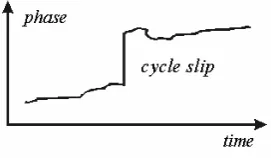
GPS receivers continuously monitor the carrier beat phase. When they lose their lock on a satellite, an unknown integer number of cycles are also lost. This event is called a 'cycle slip' (see Figure 1). These cycle slips have to be recovered in order to compute accurate positions.

The first step in the cycle slip correction consists of setting up a test quantity. Using test quantity is for eliminating the trend (geometrical distance between receiver and satellite) and time varying errors from observations, which prevents cycle slip detection. This combination has to be a slow time varying function so that a jump in this function will indicate the occurrence of a cycle slip. Formulating test quantities in the basic phase

and code measurements is needed. Selection of a special test quantity depends on the type of observations and work.

GPS observation equations are as follows [9]:

i k 1 N 1 i c k c i k i k I i k i

k 1

L =ρ − +Δρ + δ − δ +λ

i k 2 N 2 i c k c i k i k I 2 2 f

2 1 f i k i

k 2

L =ρ − +Δρ + δ − δ +λ

i c k c i k i k I i k i

k 1

P =ρ + +Δρ + δ − δ

i c k c i k i k I 2 2 f

2 1 f i k i

k 2

Figure 1. Cycle slip occurrence.

In which sub-indices 1 and 2 refers to first and second carriers and sub-indices k refers to receiver and super-indices i refer to satellite.

In general in all equations in Section 1 sub-indices k and l refer to receivers and super-sub-indices i and j refer to satellites and each quantity that has these indices it is between one or two receivers and one or two satellites.

In this paper we select the following test quantities:

• Phase-code (P. C.) combination (Range Residual) [4]:

( )

t L₁i_k

( )

t P₁i_k

( )

t ₁N₁i_k 2Ii_k

( )

t

i k 1

PC = − =λ −

( )

( )

( )

Ii_k

( )

t 2 2 f 2 1 f 2 i k 2 N 2 t i k 2 P t i k 2 L t i k 2

PC = − =λ −

• Phase-phase combination (P. P.) (Ionosphere Residual) [4]: i k 2 N 2 f 1 f i k 1 N i k I 2 2 f 2 1 f 2 2 f c 1 f 2 i k 2 L 2 f 1 f 1 i k 1 L i k PP ⎟ ⎟ ⎠ ⎞ ⎜ ⎜ ⎝ ⎛ − + ⎟ ⎟ ⎟ ⎠ ⎞ ⎜ ⎜ ⎜ ⎝ ⎛ ₋ ⎟ ⎟ ⎠ ⎞ ⎜ ⎜ ⎝ ⎛ = λ − λ =

In phase-code and phase-phase combinations some time varying errors such as satellite clock error, receiver clock error, troposphere effect and also geometric distance are eliminated. This combinations show the gradual changes of ionosphere effect from first observation epoch. Noise level of phase-code combination is high due the use of code observation. Noise level of

phase-phase combination is low.

• Melbourne-Wubbena (M. W.) linear combination [9]: ⎟ ⎠ ⎞ ⎜ ⎝ ⎛ ₋ − = ⎟ ⎠ ⎞ ⎜ ⎝ ⎛ ₊ + − ⎟ ⎠ ⎞ ⎜ ⎝ ⎛ ₋ − = i k 2 N i k 1 N 2 f 1 f c i k 2 P 2 f i k 1 P 1 f 2 f 1 f 1 i k 2 L 2 f i k 1 L 1 f 2 f 1 f 1 i k 6 L

In this combination satellite clock error, receiver clock error, troposphere effect, ionospheric effect and also geometric distance are eliminated. Noise level of this combination is not very high due to use of plus operation between two code observations that behaves as a low pass filter of code measurements. For this reason, one cycle slip is seen in this combination. If number of cycle slips in L1 and L2 are equal, are mathematically eliminated in test quantity. If the ionospheric effect is intensive, using of Melborne-Wubbena combination is proposed.

• Double difference (D. D.) observation equations [9]: ij kl 1 N 1 ij kl ij kl I ij kl ij k 1 L ij l 1 L ) i k 1 L j k 1 L ( ) i l 1 L j l 1 L ( ij kl 1 L λ + ρ Δ + − ρ = − = − − − = ij kl 2 N 2 ij kl ij kl I 2 2 f 2 1 f ij kl ij k 2 L ij l 2 L ) i k 2 L j k 2 L ( ) i l 2 L j l 2 L ( ij kl 2 L λ + ρ Δ + − ρ = − = − − − =

In this test quantity, satellite clock error and receiver clock error has been eliminated.

We can use phase-code, phase-phase and Melbourne-Wubbena combinations in single site sessions and double difference combination in two site sessions.

2. WAVELET TRANSFORMS

Figure 2. Heisenberg's uncertainty principle. series of sines and cosines. This sum is also

referred to as a Fourier expansion. The big disadvantage of a Fourier expansion, however is that it has only frequency resolution and no time resolution. This means that, although we might be able to determine all the frequencies present in a signal, we do not know when they are present. To overcome this problem in the past decades several solutions have been developed which are more or less able to represent a signal in the time and frequency domain at the same time.

The idea behind these time-frequency joint representations is to cut the signal of interest into several parts and then analyze the parts separately. It is clear that analyzing a signal this way will give more information about the time and place of different frequency components, but it leads to a fundamental problem as well: how to cut the signal? Suppose that we want to know exactly all the frequency components present at a certain moment in time. We cut out only this very short time window using a Dirac pulse; transform it to the frequency domain and so on.

The problem here is that cutting the signal corresponds to a convolution between the signal and the cutting window. Since convolution in the time domain is identical to multiplication in the frequency domain and since the Fourier transform of a Dirac pulse contains all possible frequencies, the frequency components of the signal will be smeared out all over the frequency axis. In fact this situation is the opposite of the standard Fourier transform since we now have time resolution but no frequency resolution whatsoever.

The underlying principle of the phenomena just described is due to Heisenberg's uncertainty principle, which, in signal processing terms, states that it is impossible to know the exact frequency and time of occurrence of a frequency in a signal (see Figure 2). In other words, a signal can simply not be represented as a point in the time-frequency space. The uncertainty principle shows that it is very important how one cuts the signal.

The wavelet transform or wavelet analysis is probably the most recent solution to overcome the shortcomings of the Fourier transform. In wavelet analysis the use of a fully scalable modulated window solves the signal-cutting problem. The window is shifted along the signal and for every position the spectrum is calculated. Then this

process is repeated many times with a slightly shorter (or longer) window for every new cycle. At the end, the result will be a collection of time-frequency representations of the signal, all with different resolutions. Because of this collection of representations we can speak of a multi-resolution analysis. In the case of wavelets we normally do not speak about time-frequency representations but about time-scale representations, scale being in a way the opposite of frequency, because the term frequency is reserved for the Fourier transform.

2.1. Continuous Wavelet Transform

The wavelet analysis described in the introduction is known as the continuous wavelet transform or CWT. More formally it is written as:

( )

s,τ =∫ ∞₋+_∞f

( )

t ψ*_s,τ

( )

t dt

γ (1)

Where * denotes complex conjugation. This equation shows how a function f(t) is decomposed into a set of basic functions Ψs,τ(t), called the wavelets. The variables s and τ, scale and translation, are the new dimensions after the wavelet transform.

The wavelets are generated from a single basic wavelet ψ(t), the so-called mother wavelet, by translation and scaling:

( )

⎟

⎠ ⎞ ⎜ ⎝ ⎛ −τ ψ = τ ψ

s t s 1 t ,

In (2) s is the scale factor, τ is the translation factor and the factor s-1/2 _{is for energy normalization} across the different scales.

It is important to note that in (1) and (2) the wavelet basic functions are not specified. This is a difference between the wavelet transform and the Fourier transform, or other transforms. The theory of wavelet transforms deals with the general properties of the wavelets and wavelet transforms only. It defines a framework within; one can design wavelets to own taste and wishes.

2.2. Wavelet Properties

The most important properties of wavelets are the admissibility and the regularity conditions and these are the properties which gave wavelets their name. It can be shown that square integrable functions ψ

( )

t satisfying the admissibility condition,

( )

∞ + < ω ∫ ∞+_−∞ ω ω Ψ d 2 (3)

Can be used to first analyze and then reconstruct a signal without loss of information. In (3) Ψ(ω) stands for the Fourier transform of Ψ(t). The admissibility condition implies that the Fourier transform of Ψ(t) vanishes at the zero frequency, i.e.

( )

0

0

2 ₌

= ω ω

Ψ (4)

This means that wavelets must have a band-pass like spectrum. This is a very important observation, which we will use later on, to build an efficient wavelet transform.

A zero at the zero frequency also means that the average value of the wavelet in the time domain must be zero,

( )

t dt=0

∫ ∞_{− ψ}+_∞ (5)

and therefore it must be oscillatory. In other words, Ψ(t) must be a wave.

It can be seen from (1) the wavelet transforms from a one-dimensional function to dimensional; the wavelet transform of a two-dimensional function is four-two-dimensional. The time-bandwidth product of the wavelet transform is

the square of the input signal and for most practical applications this is not a desirable property. Therefore one imposes some additional conditions on the wavelet functions in order to make the wavelet transform decrease quickly with decreasing scale s. These are the regularity conditions and they state that the wavelet function should have some smoothness and concentration in both time and frequency domains. Regularity is quite a complex concept and we will try to explain it a little, using the concept of vanishing moments. If we expand the wavelet transform (1) into the Taylor series at t = 0 until order n (let τ = 0 for simplicity) we get:

( )

( )( )

(

)

⎥ ⎥ ⎦ ⎤ ⎢ ⎢ ⎣ ⎡ ∑ = ∫ ⎟⎠ + + ⎞ ⎜ ⎝ ⎛ ψ = γ n 0

p s dt O n 1

t ! p p t 0 p f s 1 0 ,

s (6)

Here f(p) _{stands for the P}n _{derivative of f and} O(n+1) means the rest of the expansion and it is in the order of tn+1 _{when t approaches zero. Now, if} we define the moments of the wavelet about t = 0 by Mp,

( )

t dt p t p

M =∫ ∞₋+_∞ ψ (7)

Then we can rewrite (6) into the finite development

( )

( )

( )( )

( )( )

( )( )

_sn 1 _{O s}n 2 _]

n M ! n 0 n f 3 s 2 M ! 2 0 2 f 2 s 1 M ! 1 0 1 f s 0 M 0 f [ s 1 0 , s ⎟ ⎠ ⎞ ⎜ ⎝ ⎛ + + + + + + + = γ L (8) From the admissibility condition, we already have

Summarizing, the admissibility condition gave us the “wave”, regularity and vanishing moments gave us the fast decay or the “let”, and put together they give us the “wavelet”.

2.3. Discrete Wavelets

Now that we know what the wavelet transform is, we would like to make it practical. However, the wavelet transform as described so far still has three properties that make it difficult to use directly in the form of (1). The first is the redundancy of the CWT. In (1) the wavelet transform is calculated by continuously shifting a continuously scalable function over a signal and calculating the correlation between the two. It will be clear that these scaled functions will be nowhere near an orthogonal basis and the obtained wavelet coefficients will therefore be highly redundant. For most practical applications we would like to remove this redundancy.

Even without the redundancy of the CWT we still have an infinite number of wavelets in the wavelet transform and we would like to see this number reduced to a more manageable count. This is the second problem we have.

The third problem is that for most functions the wavelet transforms have no analytical solutions and they can be calculated only numerically or by an optical analog computer. Fast algorithms are needed to be able to exploit the power of the wavelet transform and it is in fact the existence of these fast algorithms that have put wavelet transforms where they are today. Let us start with the removal of redundancy.

As mentioned before the CWT maps a one-dimensional signal to a two-one-dimensional time-scale joint representation that is highly redundant. The time-bandwidth product of the CWT is the square of the signal and for most applications, which seek a signal description with as few components as possible, this is not efficient. To overcome this problem discrete wavelets have been introduced. Discrete wavelets are not continuously scalable and translatable but can only be scaled and translated in discrete steps. This is achieved by modifying the wavelet representation (2) to create

( )

⎟ ⎟ ⎟

⎠ ⎞

⎜ ⎜ ⎜

⎝

⎛ _{− τ}

ψ = ψ

j 0 s

j 0 s 0 k t j 0 s 1 t k

,j (9)

Although it is called a discrete wavelet, it normally is a (piecewise) continuous function. In (9) j and k are integers and s0 > 1 is a fixed dilation step. The translation factor τ0 depends on the dilation step. The effect of discretizing the wavelet is that the time-scale space is now sampled at discrete intervals. We usually choose s0 = 2 so that the sampling of the frequency axis corresponds to dyadic sampling. This is a very natural choice for computers, the human ear and music for instance. For the translation factor we usually choose τ0 = 1 so that we also have dyadic sampling of the time axis (see Figure 3).

When discrete wavelets are used to transform a continuous signal the result will be a series of wavelet coefficients, and it is referred to as the wavelet series decomposition. An important issue in such a decomposition scheme is of course the question of reconstruction. It is all very well to sample the time-scale joint representation on a dyadic grid, but if it will not be possible to reconstruct the signal it will not be of great use. As it turns out, it is indeed possible to reconstruct a signal from its wavelet series decomposition. It is proven that the necessary and sufficient condition for stable reconstruction is that the energy of the wavelet coefficients must lie between two positive bounds, i.e.

2 f B Z

k ,j

2 k ,j , f 2

f

A ∑

∈ ψ ≤

≤ (10)

Where f 2 is the energy of f(t), 0 < A < B, B < ∞ and A, B are independent of f(t). When (10) is satisfied, the family of basis functions ψ _,jk

( )

t with

Z k

,j ∈ is referred to as a frame with frame bounds A and B. When A = B the frame is tight. When A ≠ B exact reconstruction is still possible at the expense of a dual frame. In a dual frame discrete wavelet transform the decomposition wavelet is different from the reconstruction wavelet.

Figure 3. Localization of the discrete wavelets in the time-scale space on a dyadic grid.

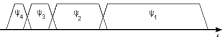
Figure 4. Touching wavelet spectra resulting from scaling of the mother wavelet in the time domain.

( )

( )

⎩ ⎨

⎧ = =

= ∫ ∞₋+_∞ψ ψ

otherwise 0

n k and m j if 1 dt t *

n , m t k

,j (11)

An arbitrary signal can be reconstructed by summing the orthogonal wavelet basis functions, weighted by the wavelet transform coefficients:

( )

∑

( )

( )

∈ ∑∈ γ ψ

= Z j k Z

t k ,j k ,j t

f (12)

Equation 12 shows the inverse wavelet transform for discrete wavelets.

Orthogonality is not essential in the representation of signals. The wavelets need not be orthogonal and in some applications the redundancy can help reducing the sensitivity to noise or improve the shift invariance of the transform. This is a disadvantage of discrete wavelets: the resulting wavelet transform is no longer shift invariant, which means that the wavelet transforms of a signal and of a time-shifted version of the same signal are not simply shifted versions of each other.

2.4. Band-Pass Filter

With the redundancy removed, we still have two hurdles to pass before we have the wavelet transform in a practical form. We continue by trying to reduce the number of wavelets needed in the wavelet transform and save the problem of the difficult analytical solutions for the end.

Even with discrete wavelets we still need an infinite number of scaling and translations to calculate the wavelet transform. The easiest way to tackle this problem is simply not to use an infinite number of discrete wavelets. Of course this poses the question of the quality of transform. Is it possible to reduce the number of wavelets to analyze a signal and still have a useful result? The translations of the wavelets are of course limited by the duration of the signal under investigation so that we have an upper boundary for the wavelets. This leaves us with the question of dilation: how many scales do we need to analyze our signal? How do we get a lower bound? It turns out that we can answer this question by looking at the wavelet transform in a different way. If we look at (4) we see that the wavelet has a band-pass like spectrum. From Fourier theory we know that compression in time is equivalent to

stretching the spectrum and shifting it upwards:

( )

{

}

⎟

⎠ ⎞ ⎜ ⎝ ⎛ ω =

a F a 1 at f

F (13)

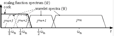
Figure 5. How an infinite set of wavelets is replaced by one scaling function.

2.5. The Scaling Function

How to cover the spectrum all the way down to zero? Because every time you stretch the wavelet in the time domain with a factor of 2, its bandwidth is halved. In other words, with every wavelet stretch you cover only half of the remaining spectrum, which means that you will need an infinite number of wavelets to get the job done.

The solution to this problem is simply not to try to cover the spectrum all the way down to zero with wavelet spectra, but to use a cork to plug the hole when it is small enough. This cork then is a low-pass spectrum and it belongs to the so-called scaling function. The scaling function was introduced by Mallat. Because of the low-pass nature of the scaling function spectrum it is sometimes referred to as the averaging filter. If we look at the scaling function as being just a signal with a low-pass spectrum, then we can decompose it in wavelet components and express it like:

( )

∑

( )

( )

∈ ∈∑ γ ψ

= ϕ

Z

j k Z ,jk ,jk t

t (14)

Since we selected the scaling function ϕ

( )

t in such a way that its spectrum neatly fitted in the space left open by the wavelets, the expression (14) uses an infinite number of wavelets up to a certain scale j (see Figure 5). This means that if we analyze a signal using the combination of scaling function and wavelets, the scaling function by itself takes care of the spectrum otherwise covered by all the wavelets up to scale j, while the rest is done by the wavelets. In this way we have limited the number of wavelets from an infinite number to a finite number.

By introducing the scaling function we have circumvented the problem of the infinite number of wavelets and set a lower bound for the wavelets.

Of course, when we use a scaling function instead of wavelets we lose information. That is to say, from a signal representation point of view we do not lose any information, since it will still be possible to reconstruct the original signal, but from a wavelet-analysis point of view we discard possible valuable scale information. The width of the scaling function spectrum is therefore an important parameter in the wavelet transform design. The shorter its spectrum the more wavelet coefficients you will have and the more scale information. But, as always, there will be practical limitations on the number of wavelet coefficients you can handle. As we will see later on, in the discrete wavelet transform this problem is more or less automatically solved.

The low-pass spectrum of the scaling function allows us to state some sort of admissibility condition similar to (5)

( )

t dt=1

∫ ∞_{− ϕ}+_∞ (15)

Which shows that the 0th _{moment of the scaling} function can not vanish.

Summarizing once more, if one wavelet can be seen as a band-pass filter and a scaling function as a low-pass filter, then a series of dilated wavelets together with a scaling function can be seen as a filter bank.

2.6. Sub-Band Coding

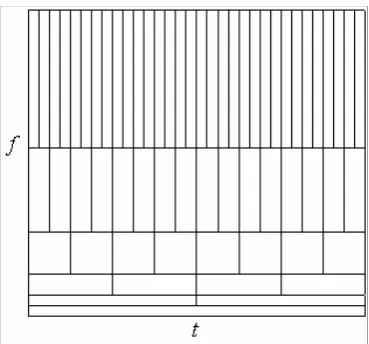
Two of the three problems mentioned in Section 2.3 have now been resolved, but we still do not know how to calculate the wavelet transform. Therefore we will continue our discussion through multi-resolution land. If we regard the wavelet transform as a filter bank and then we can consider wavelet transforming a signal as passing the signal through this filter bank. The outputs of the different filter stages are the wavelet-and scaling function transform coefficients. Analyzing a signal by passing it through a filter bank is not a new idea and has been around for many years under the name sub-band coding. It is used for instance in computer vision applications.

Figure 6. Splitting the signal spectrum with an iterated filter bank.

of every band can be chosen freely, in such a way that the spectrum of the signal to analyze is covered in the places where it might be interesting. The disadvantage is that we will have to design every filter separately and this can be a time consuming process. Another way is to split the signal spectrum in two (equal) parts, a low-pass and a high-pass part. The high-pass part contains the smallest details we are interested in and we could stop here. We now have two bands. However, the low-pass part still contains some details and therefore we can split it again. And again, until we are satisfied with the number of bands we have created. In this way, we have created an iterated filter bank. Usually the number of bands is limited by, for instance, the amount of data or computation power available. The process of splitting the spectrum is graphically displayed in Figure 6. The advantage of this scheme is that we have to design only two filters; the disadvantage is that the signal spectrum coverage is fixed.

Looking at Figure 6 we see that what we are left with after the repeated spectrum splitting is a series of band-pass bands with doubling bandwidth and one low-pass band. (Although in theory the first split gave us a high-pass band and a low-pass band, in reality the high-pass band is a band-pass band due to the limited bandwidth of the signal.) In other words, we can perform the same sub-band analysis by feeding the signal into a bank of band-pass filters of which each filter has a bandwidth twice as wide as his left neighbor (the frequency axis runs to the right here) and a low-pass filter. At the beginning of this section we stated that this is the same as applying a wavelet transform to the signal. The wavelets give us the band-pass bands

with doubling bandwidth and the scaling function provides us with the low-pass band. From this we can conclude that a wavelet transforms is the same thing as a sub-band coding scheme using a constant-Q filter bank. In general we will refer to this kind of analysis as a multi-resolution analysis. Summarizing, if we implement the wavelet transform as an iterated filter bank, we do not have to specify the wavelets explicitly! This sure is a remarkable result.

2.7 Discrete Wavelet Transform

In many practical applications the signal of interest is sampled. In order to use the results we have achieved so far with a discrete signal and we have to make our wavelet transform discrete, too. We remember that our discrete wavelets are not time-discrete, only the translation-and the scale step are discrete. Simply implementing the wavelet filter bank as a digital filter bank intuitively seems to do the job.

In (14), we stated that the scaling function could be expressed in wavelets from minus infinity up to a certain scale j. If we add a wavelet spectrum to the scaling function spectrum we will get a new scaling function, with a spectrum twice as wide as the first. The effect of this addition is that we can express the first scaling function in terms of the second, because all the information we need to do this is contained in the second scaling function. We can express this formally in the so-called multi-resolution formulation or two-scale relation:

( )

∑

∈ ⎟⎠

⎞ ⎜

⎝

⎛ + ₋

ϕ + =

⎟ ⎠ ⎞ ⎜ ⎝ ⎛ ϕ

Z k

k t 1 j 2 k 1 j h t

j

2 (16)

The two-scale relation states that the scaling function at a certain scale can be expressed in terms of translated scaling functions at the next smaller scale. Smaller scale means more detail. The first scaling function replaced a set of wavelets and therefore we can also express the wavelets in this set in terms of translated scaling functions at the next scale. More specifically we can write for the wavelet at level j:

( )

∑

∈ ⎟⎠

⎞ ⎜

⎝

⎛ + ₋

ϕ + =

⎟ ⎠ ⎞ ⎜ ⎝ ⎛ ψ

Z

k t k

1 j 2 k 1 j g t

j

2 (17)

function and the wavelet.

Since our signal f(t) could be expressed in terms of dilated and translated wavelets up to a scale j-1, this leads to the result that f(t) can also be expressed in terms of dilated and translated scaling functions at a scale j:

( )

∑

( )

∈ ⎟⎠ ⎞ ⎜ ⎝ ⎛ ₋ ϕ λ = Z k k t j 2 k j t

f (18)

To be consistent in our notation we should in this case speak of discrete scaling functions since only discrete dilations and translations are allowed. If in this equation we step up a scale to j-1, we have to add wavelets in order to keep the same level of detail. We can then express the signal f(t) as

( )

( )

( )

∑ ∈ ⎟⎠ ⎞ ⎜ ⎝ ⎛ − ₋ ψ − γ + ∑ ∈ ⎟⎠ ⎞ ⎜ ⎝ ⎛ − ₋ ϕ − λ = Z

k t k

1 j 2 k 1 j Z k k t 1 j 2 k 1 j t f (19)

If the scaling function ϕ_,jk

( )

t and the wavelets

( )

t k ,j

ψ are orthonormal or a tight frame, then the coefficients λ_j−1

( )

k and γ_j−1

( )

k are found by taking the inner products

( )

( )

( )

( )

k f

( )

t, _,jk

( )

t

1 j t k ,j , t f k 1 j ψ = − γ ϕ = − λ (20)

If we now replace ϕ_,jk

( )

t and ψ _,jk

( )

t in the inner products by suitably scaled and translated versions of (16) and (17) and manipulate a bit, keeping in mind that the inner product can also be written as an integration, we arrive at the important result:

( )

∑

(

) ( )

∈ − λ

= − λ

Z

m h m 2k j m k

1

j (21)

( )

∑

(

) ( )

∈ − γ

= − γ

Z

m g m 2k j m k

1

j (22)

These two equations state that the wavelet- and scaling function coefficients on a certain scale can be found by calculating a weighted sum of the

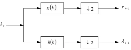
scaling function coefficients from the previous scale (see Figure 7). Now recall from the section on the scaling function that the scaling function coefficients came from a low-pass filter and recall from the section on sub-band coding how we iterated a filter bank by repeatedly splitting the low-pass spectrum into a low-pass and a high-pass part. The filter bank iteration started with the signal spectrum, so if we imagine that the signal spectrum is the output of a low-pass filter at the previous (imaginary) scale, then we can regard our sampled signal as the scaling function coefficients from the previous (imaginary) scale. In other words, our sampled signal f(k) is simply equal to λ(k) at the largest scale!

But there is more. As we know from signal processing theory a discrete weighted sum like the ones in (21) and (22) is the same as a digital filter and since we know that the coefficients λj(k) come from the low-pass part of the splitted signal spectrum, the weighting factors h(k) in (21) must form a low-pass filter. And since we know that the coefficients γj(t) come from the high-pass part of the splitted signal spectrum, the weighting factors g(k) in (22) must form a high-pass filter. This means that (21) and (22) together form one stage of an iterated digital filter bank and from now on we will refer to the coefficients h(k) as the scaling filter and the coefficients g(k) as the wavelet filter. By now we have made certain that implementing the wavelet transform as an iterated digital filter bank is possible and from now on we can speak of the discrete wavelet transform or DWT. Our intuition turned out to be correct. Because of this we are rewarded with a useful bonus property of (21) and (22), the sub-sampling property. If we take one last look at these two equations we see that the scaling and wavelet filters have a step-size of 2 in the variable k. The effect of this is that only every other λj(k) is used in the convolution, with the result that the output data rate is equal to the input data rate. Although this is not a new idea, it has always been exploited in sub-band coding schemes, it is kind of nice to see it pop up here as part of the deal.

( )

k g

( )k h

j λ

2

↓

2

↓ γj−1

1

−

j λ

Figure 7. Implementation of (21) and (22) as one stage of an iterated filter bank.

Figure 8. Db1 wavelet (Haar's wavelet). number of samples for the next stage is halved so

that in the end we are left with just one sample (in the extreme case). It will be clear that this is where the iteration definitely has to stop and this determines the width of the spectrum of the scaling function. Normally the iteration will stop at the point where the number of samples has become smaller than the length of the scaling filter or the wavelet filter, whichever is the longest, so the length of the longest filter determines the width of the spectrum of the scaling function.

So we have managed to reduce the highly redundant continuous wavelet transform as formulated in (1) with its infinite number of unspecified wavelets to a finite stage iterated digital filter bank which can be directly implemented on a digital computer. The redundancy has been removed by using discrete wavelets and a scaling function solved the problem of the infinite number of wavelets needed in the wavelet transform. The filter bank has solved the problem of the non-existence of analytical solutions as mentioned in the section on discrete wavelets. Finally, we have built a digitally implementable version of (1) without specifying any wavelet, just as in (1). The wavelet transform has become very practical indeed.

3. CYCLE SLIP DETECTION USING WAVELET TRANSFORMS

Wavelet transform could be done in two forms: Continuous wavelet transform and discrete wavelet transform. Detection of cycle slip using wavelet transform could be explained as follows:

Indeed the continuous wavelet transform is the inner product of the time series of test quantity and the scaled, shifted versions of wavelet function, so the resulting coefficients from continuous wavelet transform show the similarity between time series of test quantity and the wavelet. It should be noted that for calculation of continuous wavelet transform coefficients we have to use the small values for scale because cycle slip is a high frequency phenomena.

In order to detect the cycle slip using discrete wavelet transform, we apply two high pass filter and low pass filter on time series of test quantity.

Resulting coefficients from low pass filter show the general figure (approximation) of the signal and resulting coefficients from high pass filter show the details or high frequencies of the signal, so existence of jump in the output of high pass filter shows the place of cycle slip occurrence in GPS observables.

3.1. Selection of a Appropriate Wavelet

The

characteristic of cycle slip is a discontinuity in the epoch of cycle slip and the amplitude of slip give us information about the value of cycle slip.

Owing to the fact that the wavelet transform detects only parts of the signal similar to itself, a wavelet looks like the discontinuities encountered in the GPS observations should be selected.

For this purpose the low order Daubechies's wavelets (db1 and db2 wavelets) were used. Selection of these wavelets is due to their shape and compact support.

( )

[

[

( )

[

[

( )

[ [

( )

[ [

( )

t 0, if t

[ [

0,1

1 , 0 t if

, 1 t

1 , 0 t if

, 0 t

1 , 5 . 0 t if

, 1 t

5 . 0 , 0 t if

, 1 t

∉ =

φ

∈ =

φ

∉ =

ψ

∈ −

= ψ

∈ =

ψ

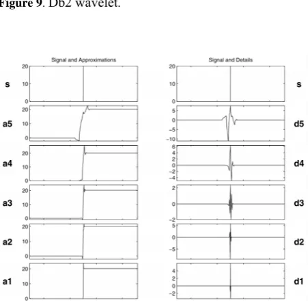
The GPS carrier beat phase has a parabolic behavior due to the Doppler Effect. In order to eliminate the parabolic behavior introduced in the wavelet transform the Haar wavelet is not proper. This wavelet was built to detect jumps versus a horizontal right line. The parabolic behavior of the signal is seen by this wavelet as a succession of jumps (see Figures 20a and 20b). The wavelet to be used will detect jumps versus a parabola. So we should use a wavelet that removes the parabolic behavior of the GPS signal. For this purpose, according to the following theorem, we used from db2 wavelet that was built by Ingrid Daubechies. 3.1.1. Theorem “Every dbN wavelet has N vanishing moment” [8].

So db2 wavelet detects cycle slips in the first derivative of the signal and the parabolic behavior is removed from the wavelet transform of the signal (see Figure 9).

After cycle slip detection we try to determine the value of cycle slip using wavelet transforms. For this purpose we apply discrete wavelet transform on phase-code combination, then fitting a low order polynomial on the output of low pass filter. The resulting values for cycle slip could be precized using phase-phase combination.

3.2. Wavelet Transform of a Signal with a

Discontinuity

One of the major applications of

wavelet transforms is detection of discontinuity place in the signal because these transforms provide the joint time-frequency representation of signal.

According to the Heisenberg's uncertainty principle (see Figure 2), using the wavelet transform in high frequencies has good time resolution, contrary to low frequencies. Because cycle slip is a high frequency phenomenon in the time series of observations or test quantities, wavelet transforms can precisely detect the place of cycle slip in the signal.

Here we are faced with the simplest example of

a rupture (i.e., a step, see Figure 10). We did a discrete wavelet transform with db2 wavelet using 5 decomposition levels. The time instant when the jump occurs is equal to 500. The break is detected at all levels, but it is obviously detected with greater precision in the higher resolutions (levels 1 and 2) than in the lower ones (levels 4 and 5). It is very precisely localized at level 1, where only a very small zone around the jump time can be seen. It should be noted that the reconstructed details are primarily composed of the basic wavelet represented in the initial time. Furthermore, the rupture is more precisely localized when the wavelet corresponds to a short filter [7].

In the above figure discontinuity not only is seen in the high pass filter output but also in the low pass filter output and in the successive decomposition levels this is true. The reason is that the cycle slip causes a discontinuity in the test quantity that is seen as a step. A look at the spectrum of the step function in frequency domain shows that it contains all possible frequencies, so it is seen in the output of both filters.

Figure 9. Db2 wavelet.

Figure 10. Wavelet transform of a signal with a discontinuity at t = 500, analyzing wavelet: db2, decomposition levels: 5.

Figure 11. Discrete wavelet transform of a signal with a polynomial and white noise, analyzing wavelets: db2 and db3,

decomposition levels: 4. Figure 12. Selection of applied data.

play in any of the details. The wavelet suppresses the polynomial part and analyzes the noise [7].

4. EXPERIMENT RESULTS

4.1. Isun1 Package

This package is prepared in

Tabriz University for special studies in GPS.

4.2. Applied Data

Shown in Figure 12 is the test data that used here. N. C. C. GPS group has collected data at 18 March 2001 for 2 hours with LEICA SR299 receivers. The observations recording are made every 3 seconds.

Processing results using Geogenius software showed that CNCO and DNCO stations observations to satellites no 2 and 7 is free from cycle slips. In single site experiment we simulated artificial cycle slips in the observations from CNCO station to satellite no 2 (see Table 1). In two site experiment we simulated artificial cycle slips in the observations from CNCO and DNCO stations to satellites no 2 and 7 (see Tables 2 to 5).

4.3. Results of Program in Test Data

We made different test quantities from observations and applied discrete wavelet transforms on them. Figure 13a shows P. C. 1 combination without cycle slip. Figure 13b shows this combination with simulated cycle slips.

TABLE 1. Simulated Cycle Slips in phase Observations from CNCO Station to PRN No. 2 in Single Site Experiment.

TABLE 2. Simulated Cycle Slips in Phase Observations from CNCO Station to PRN No. 2.

TABLE 3. Simulated Cycle Slips in Phase Observations from CNCO Station to PRN No. 7.

TABLE 4. Simulated Cycle Slips in Phase Observations from DNCO Sation to PRN No. 2.

TABLE 5. Simulated Cycle Slips in Phase Observations from DNCO Station to PRN No. 7.

(a)

(b)

Figure 13. (a) P. C. 1 combination without cycle slip, (b) P. C. 1 combination with cycle slip.

simulated cycle slips are not identifiable. Figures 14a and 14b show the high pass filter output of discrete wavelet transform of phase-code combination using db1 wavelet. Comparison of theses figures show that the noise level of this combination is of the order of one Li cycle so cycle slips in 500 and 1500 epochs are not detected, but

cycle slips in 1000, 2000 and 2500 epochs are detected. Larger values (5 to 10 cycles) are observed in the case of multipath, and for low elevations. As a consequence, this method only gives a first approximation of the jumps.

(a)

(b)

Figure 14. (a) High-pass filter output of W. T. of P. C. 1 combination without cycle slip, (b) High-pass filter output of W. T. of P. C. 1 combination with cycle slip.

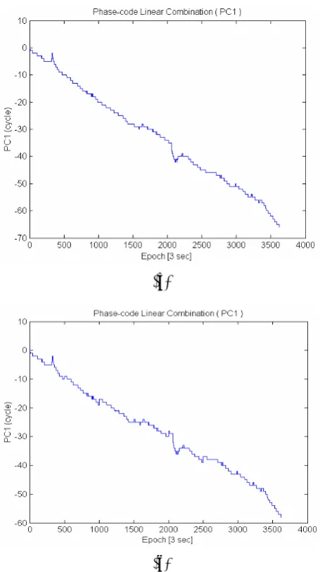
(a)

(b)

Figure 15. (a) P. P. combination without cycle slip, (b) P. P. combination with cycle slip.

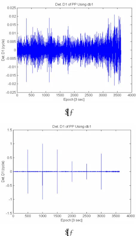
Figures 16a and 16b show the high pass filter output of discrete wavelet transform of phase-phase combination using db1 wavelet. Comparison of these figures shows that all cycle slips have been detected.

Figure 17a shows the Melbourne-Wubbena combination without cycle slip. Figure 17b shows this combination with simulated cycle slips.

Figures 18a and 18b show the high pass filter output of discrete wavelet transform of Melbourne-Wubbena combination using db1 wavelet. Comparison of these figures shows that the noise

level of this combination is less than one cycle. Cycle slip in 2500 epoch number is not detected, because in this epoch the number of cycle slips is equal in both carriers and mathematically eliminated in test quantity.

(a)

(b)

Figure 16. (a) High-pass filter output of W. T. of P. P. combination without cycle slip, (b) High-pass filter output of W.T. of P. P. combination with cycle slip.

(a)

(b)

Figure 17. (a) M. W. combination without cycle slip, (b) M. W. combination with cycle slip.

trend due to Doppler Effect is apparent from Figures 19a and 19b.

For cycle slip detection, in the first step we did the discrete wavelet transform using db1 wavelet. Figures 20a and 20b show that this trend has appeared as successive jumps in the high-pass filter output of discrete wavelet transform and detection has not done successfully.

In order to elimination of this trend we chose db2 wavelet. Figures 21a and 21b show the high-pass filter outputs of discrete wavelet transform of this combination using db2 wavelet. These figures

show that the parabolic trend has been eliminated in this transform and simulated cycle slips have been detected successfully.

5. CONCLUSIONS AND RECOMMENDATIONS

The aim of this paper was to demonstrate that the wavelet transform can be used to detect cycle slips in GPS measurements.

(a)

(b)

Figure 18. (a) High-pass filter output of W. T. of M. W. combination without cycle slip, (b) High-pass filter output of W. T. of M. W. combination with cycle slip.

(a)

(b)

Figure 19. (a) D. D. observations without cycle slip, (b) D. D. observations with cycle slip.

function, the Haar wavelet (db1) is a good basis to approximate this function. For cycle slip detection from P. C. and P. P. combinations the db1 wavelet is the best. Db2 wavelet can also follow the jump in the first order derivative of the signal. For this reason, cycle slip detection from D. D. combination using the db2 wavelet is proposed.

In general for GPS data processing the low order compact support Daubechies’s wavelets are recommended. The choice is based on the following reasons: the short wavelet basis has less phase distortion and time delay to facilitate a good signal recovery in real time.

The advantage of the wavelet transform method lies in the fact that the filter is easy to implement. It is very precise in the time location of a cycle slip.

The disadvantages of this method are; (1) The filter is a non-adaptive one, (2) A signal with a lot of noise can be seen as successive jumps.

In general due to the redundancy problem of continuous wavelet transform, using discrete wavelet transform in GPS data processing is recommended.

(a)

(b)

Figure 20. (a) High-pass filter output of W. T. of D. D. combination without cycle slip using db1, (b) High-pass filter output of W. T. of D. D. combination with cycle slip using db1.

(a)

(b)

Figure 21. (a) High-pass filter output of W. T. of D. D. combination without cycle slip using db2, (b) High-pass filter output of W. T. of D. D. combination with cycle slip using db2.

of the observations, state-transition noise matrix. The Kalman filter is very sensitive to these a priori values. Ideally, they should be adapted to the different situations that can be encountered: these values vary in function of the receiver type, multipath, the ionosphere conditions and so on. However, a suitable choice of these initial conditions will give a powerful tool to study a signal deteriorated by noise. The wavelet transform does not need any a priori value, is very simple to implement but does not give as good results as the Kalman filter on noisy signals.

As a consequence, the two mathematically independent methods seem to be very complementary and should be used together to give mutual confirmation of the computed cycle slips.

If we don't have any information about the covariance matrix of observations, accurate detection of simulated cycle slip using Kalman filtering via arbitrary values for this matrix, can give us a good idea about this matrix.

transforms. The precision of GPS code measurements can be increased by wavelet denoising techniques. For static and low dynamic receivers, the receiver state information is confined in a very narrow low frequency band and the denoising signal is directly derived from the output of the corresponding low-pass filter bank (data smoothing).

Wavelet transforms can be used to separate multipath from the signal. The signal is double differential phase observation, which is an input for wavelet transform system. Through multi-step decomposition for original double differential observation, multipath identity is exhibited at a certain scale in the decomposition and the double differential observation is then reconstructed by a filtering to the signal with multipath eliminated. The newly formed observation is then used as the input for baseline adjustment unit to achieve desired positioning efficiency.

It is important to transmitting the measurement information to and from reference and multi-user stations quickly for real time DGPS navigation. Transmitting a compressed data perhaps is one of the best choice means (data compression). The GPS data compression can be derived directly from the fast wavelet transform algorithm. Firstly, the compression is by denoising and bias elimination; secondly because the GPS measurements are closed-correlated, the redundancy of information is reduced by the orthogonal projection of the signal to the orthogonal space spanned by orthonormal wavelets.

6. LIST OF SYMBOLS

i k

L Phase pseudorange between satellite receiver k in meters

i k

P Code pseudorange between satellite i and receiver k in meters

i k

ρ Geometric distance between satellite i and receiver k

i k

I Ionospheric refraction between

satellite i and receiver k

i k ρ

Δ Tropospheric refraction between satellite i and receiver k

c Velocity of light

δk Clock error of receiver k δi _{Clock error of satellite i} λ Wavelength

f Carrier frequency

N Phase ambiguity

7. REFERENCES

1. Bastos, L. and Landau, H., “Fixing Cycle Slip in Dual Frequency Kinematic GPS Applications Using Kalman Filtering”, Manuscripta Geodetica, Vol. 13, (1998),

249-256.

2. Daubechies, I., “Ten Lectures on Wavelets”, CBMS Series, Philadelphia, Pennsylvania, SIAM,(1992), 357. 3. Goad, C., “Precise Positioning with the Global

Positioning”, Proceedings of the Third International Symposium on Inertial Technology for Surveying and Geodesy, Banff, Canada, (September 16-20, 1985), 745-756.

4. Hofmann-Wellenhof, B., Lichtenegger, H. and Collins, J., “GPS Theory and Practice”, 4th _Edition, Springer-Verlag, Wien, (1997), 389.

5. Kaiser, G., “A Friendly Guide to Wavelets”, Boston, Birkhäuser, (1994).

6. Leick, A., “GPS Satellite Surveying”, 2nd Edition, John Wiley and Sons, Inc., New York, U.S.A., (1995), 560. 7. Misiti, M., Misiti, Y., Oppenheim, G. and Poggi, J. M.,

“Wavelet Toolbox: for Use with Matlab”, The Mathworks, Inc., Natick, Massachusetts, U.S.A., (March 1996).

8. Rastbood, A., “Detection and Solution of GPS Cycle Slip with Wavelet Transforms and Comparison with Kalman Filtering”, M.Sc. Thesis in Geodesy K. N. Toosi University of, Faculty of Geodesy and Geomatics ENG, Tehran, Iran, (2001).

9. Rothacher, M., Mervart, L., Beutler, G., Brockmann, E., Fankhauser, S., Gurtner, W., Johnson, J., Schaer, S., Springer, T. and Weber, R., “Bernese GPS Software Version 4.0”, Astronomical Institute of the University of Berne, Berne, Switzerland, (September 1996).

10. Seeber, G., “Satellite Geodesy”, Walter de Gruyter and Co., Berlin, (1993), 531.