F U L L P A P E R
Open Access
High-latitude GPS phase scintillation and cycle
slips during high-speed solar wind streams and
interplanetary coronal mass ejections: a superposed
epoch analysis
Paul Prikryl
1*, P Thayyil Jayachandran
2, Sajan C Mushini
3and Ian G Richardson
4,5Abstract
Results of a superposed epoch (SPE) analysis of occurrence of phase scintillation and cycle slips at high latitudes keyed by arrival times of high-speed solar wind streams (HSS) and interplanetary coronal mass ejections (ICME) for years 2008 to 2012 are presented. Phase scintillation indexσΦis obtained in real time from L1 signal recorded at the rate of 50 Hz by specialized global positioning system (GPS) ionospheric scintillation and total electron content (TEC) monitors (GISTMs) deployed as a part of the Canadian High Arctic Ionospheric Network (CHAIN). The phase scintillation, mapped as a function of magnetic latitude and magnetic local time, occurs predominantly on the dayside in the cusp and in the nightside auroral oval. The scintillation occurrence peaks on days of HSS or ICME impacts at the Earth's magnetosphere and tapers off a few days later, which is similar to day-to-day variability of geomagnetic activity and riometer absorption at high latitudes. ICMEs that are identified as magnetic clouds are significantly more geoeffective than HSSs and ICMEs with no or weak magnetic cloud characteristics. On their arrival day, magnetic clouds result in higher occurrence, and thus probability, of scintillation in the nightside auroral zone. The SPE analysis results are used to obtain cumulative probability distribution functions for the phase scintillation occurrence that can be employed in probabilistic forecast of phase scintillation at high latitudes.
Keywords:Ionosphere; Ionospheric irregularities; GPS scintillation; Solar wind disturbances; Space weather forecasting
Background
Ionospheric scintillation (Aarons 1982, 1997; Aarons et al. 2000; Basu et al. 1987, 1995, 1998) of the Global Navigation Satellite Systems (GNSS) signal severely de-grades positional accuracy, causes cycle slips which can lead to loss of lock, and affects performance of radio communications and navigation systems. GNSS receiver tracking performance during severe scintillation condi-tions can be assessed by the analysis of receiver phase-locked-loop (PLL) jitter (Conker et al. 2003; Sreeja et al. 2011). At high latitudes, statistical characterization and climatology of scintillation of global positioning system (GPS) signals show prevalence of phase over amplitude
scintillation with the phase scintillation primarily caused by steep ionospheric density gradients and irregularities associated with auroral and cusp precipitation and polar cap patches (Spogli et al. 2009; Li et al. 2010; Prikryl et al. 2011a, b, 2013a; Jiao et al. 2013). The ionospheric dynamics in these regions is driven by the coupling be-tween solar wind, the magnetosphere, and ionosphere. Solar wind disturbances, in particular, the co-rotating interaction regions (CIRs) on the leading edge of high-speed streams (HSSs) and interplanetary coronal mass ejections (ICMEs) have been closely linked with the oc-currence of scintillation at high latitudes (Prikryl et al. 2012). These initial results demonstrated a technique of probabilistic forecast of phase scintillation occurrence in the cusp relative to arrival times of CIRs and ICMEs. Such scintillation prediction can be combined with as-sessment of the GNSS receiver tracking performance
* Correspondence:[email protected] 1
Geomagnetic Laboratory, Natural Resources Canada, 2617 Anderson Rd, Ottawa, ON K1A 0E7, Canada
Full list of author information is available at the end of the article
(Prikryl et al. 2013b) and thus offer a potentially useful tool to provide users with expected tracking conditions. In this paper, we extended the superposed epoch (SPE) analysis of solar wind parameters and scintillation occur-rence over a period of 5 years (2008 to 2012) and ob-tained probability distribution functions that can be used in probabilistic forecasting of phase scintillation and cycle slip occurrence at high latitudes.
Methods
Phase scintillation data used in this study were collected from 2008 and 2012 by ten specialized GPS ionospheric scintillation and total electron content (TEC) monitors (GISTMs) of the Canadian High Arctic Ionospheric Network (CHAIN) (http://chain.physics.unb.ca/chain) (Jayachandran et al. 2009). CHAIN instruments, includ-ing six ionosondes, are distributed in the auroral oval, cusp, and the polar cap (Figure 1). A brief description of CHAIN, the scintillation parameters obtained, and the geographic and corrected geomagnetic coordinates of stations can be found in Prikryl et al. (2011a).
The NovAtel OEM4 GSV 4004B dual frequency GPS receivers (Van Dierendonck and Arbesser-Rastburg 2004), with special firmware specifically configured to record the power and phase of the L1 signal at 50-Hz sampling rate, compute the ionospheric TEC using both L1 and L2 sig-nals, the amplitude scintillation index S4, and the phase
scintillation index σΦ. The phase scintillation index σΦ is the standard deviation of the detrended phase using a filter in the receiver with 0.1-Hz lower cutoff. Intense scintilla-tion is usually accompanied by cycle slips. A cycle slip
(Horvath and Crozier 2007) is defined here as a jump in differential phase TEC of more than or equal to 1.5 TECU in 1 s (1 TEC unit corresponds to 1016electrons/m2).
Solar wind data, projected to the Earth's bow shock, are obtained from the Goddard Space Flight Center Space Physics Data Facility OMNIWeb (http://omniweb. gsfc.nasa.gov/). To characterize the solar wind by one index, we use the quasi-invariant (QI) index (Osherovich et al. 1999) that is defined as the ratio of the solar-wind magnetic to ram pressures.
High-speed streams generate CIRs, regions between the fast and slow solar wind where the solar wind plasma is compressed. Following the criteria of (Prikryl et al. 2012), arrival times of high-speed stream interfaces CIR/HSSs are determined. A total of 108 HSS/CIRs with a maximum velocityVMAXexceeding 500 km/s are used
in the SPE analysis of scintillation data from 2008 to 2012. For ICMEs, we use a catalogue of near-Earth ICMEs (Richardson and Cane 2010) that is updated at http://www.srl.caltech.edu/ACE/ASC/DATA/level3. In this table, ICMEs are classified into three categories based on the properties of magnetic clouds in column l: a value of 2 in this column indicating that a magnetic cloud (MC) has been reported in association with the ICME; a value of 1 indicating that the ICME shows evidence of a rotation in field direction but lacks some other characteristics of an MC, for example, an enhanced magnetic field; and a value of 0 indicating that the ICME has not been a reported magnetic cloud and lacks most of the typical features of a magnetic cloud, such as a smoothly rotating, enhanced magnetic field.
The time of the leading edge (front) of an HSS or of the ICME upstream shock/wave/disturbance provides key times of a geoeffective solar wind disturbance ob-served upstream from the Earth. Projected to the Earth's bow shock (OMNI), these key arrival times can be used in an SPE analysis to obtain an average response of the ionosphere, e.g., geomagnetic disturbance (McPherron and Siscoe 2004; McPherron and Weygand 2006), riometer absorption (Kavanagh et al. 2012), and scintilla-tion and cycle slip occurrence (Prikryl et al. 2012). Such results can then be used in probabilistic forecasting of a given ionospheric variable due to specific solar wind conditions. This can be thought of as an analogy to traditional meteorology approach in weather forecasting based on atmospheric air mass climatologies separated by boundaries (weather fronts) as discussed by McPherron and Siscoe (2004).
SPE analysis of solar wind and scintillation data
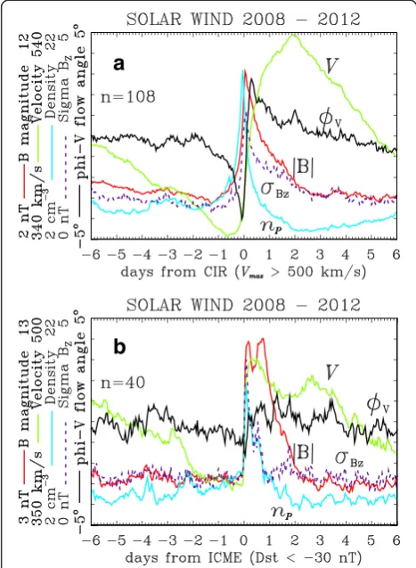
To obtain the mean variations of solar wind parameters relative to HSS interface (CIR) SPE analysis of solar wind plasma time series is performed. Figure 2a shows the mean solar wind velocity,V, mean flow angleΦV, density, Figure 1Canadian High Arctic Ionospheric Network (CHAIN).
np, magnetic field magnitude, |B|, and standard
devi-ation of IMF BZ component,σBz, over 12 days centered
at the key time (day 0). The mean solar wind velocity de-creases to a minimum just before the stream interface and then steeply rises to a maximum 2 days later. All other mean solar wind parameters peak at, or very close to, the key time. The mean flow angleΦVshows a
bipo-lar east-west deflection. Figure 2b shows the results of the SPE analysis for 40 ICMEs for which the geomag-netic disturbance, Dst, was less than −30 nT. Because the ICMEs are often preceded by shocks, the mean V, np, |B|, and σBz increase near the key time. The mean
flow angleΦVdoes not show a strong bipolar east-west
deflection that is typical for CIRs. These results are simi-lar to those obtained previously (Prikryl et al. 2012) for 2008 to 2010.
The GPS phase scintillation predominantly occurs in the ionospheric footprint of the cusp, auroral oval, and polar cap (Spogli et al. 2009; Prikryl et al. 2011a, b, 2012). In response to varying geomagnetic activity, the
scintillation regions shift in latitude. To examine a re-sponse of scintillation and to propose a method of scin-tillation forecasting relative to arrival time of CIRs and ICMEs, Prikryl et al. (2012) focused on the cusp stations in Cambridge Bay and Taloyoak that showed steep in-creases in scintillation occurrence on the zero epoch day tapering off a few days later. We now include ten CHAIN stations in the SPE analysis. The scintillation and cycle slip occurrence is mapped as a function of CGM latitude and magnetic local time (MLT).
Similarly to solar wind parameters in Figure 2, Figure 3a,b shows the SPE analysis results for QI and Kp indices, shown in green and black lines, respectively. The mean QI index increases more gradually and peaks later but reaches a higher value for ICMEs than for HSS/CIRs. This is be-cause many ICMEs are actually magnetic clouds, and the ratio of the magnetic to ram pressures is higher inside the magnetic cloud. Also, the average background levels of QI
a
b
Figure 2Superposed epoch analysis of solar wind plasma parameters.VelocityV, densitynp, magnetic field magnitude |B|,
standard deviation of the IMFBZcomponentσBz, and mean flow
angleϕVare keyed by the arrival times of(a)major CIRs and(b)
ICMEs. The scale ranges and colors/line styles for each parameter are shown in the label for the ordinate.
a
b
Figure 3Superposed epoch analysis.QI (green line),Kp(black line), number of cycle slipsNcys(red dotted line), and phase
and Kpbefore the arrival of a solar wind disturbance are higher for ICMEs than for HSS/CIRs because most of the ICMEs occurred in the years of rising solar activity (2010 to 2012), while the HSS/CIRs events are distributed more evenly over the whole period. However, the focus of this study is phase scintillation occurrence and number of cycle slipsNcysthat are shown in Figure 3a,b in blue and
red lines, respectively. They are averaged over the cusp re-gion defined here by latitude range from 70.0°N to 82.5°N and MLT from 0600 to 1800 hours. Both the scintillation and cycle slip occurrence peaked about three to four times higher for ICMEs than for HSS/CIRs. As we already noted for QI and Kp indices, the background average levels of occurrences are higher for the case of ICMEs than for HSS/CIRs.
Figures 4 and 5 show the SPE analysis results for CIRs and ICMEs, respectively, for all magnetic latitudes and MLTs. Figure 4a,b shows the SPE analysis results based on 108 CIRs, namely, the maps of percentage occurrence of phase scintillationσΦexceeding 0.1 radians and aver-age number of cycle slips, respectively. The positions of the statistical auroral oval (Feldstein and Starkov 1967; Holzworth and Meng 1975) are superposed in white line for conditions from very quiet (IQ = 0) to disturbed (IQ = 6), proportionally to the daily mean value of the Kpindex. For each epoch day, the phase scintillation oc-currence and mean number of cycle slips maximized in the cusp and extended into the polar cap with the grand maximum occurring on the epoch day 0. However, sig-nificant scintillation also occurred at auroral and even at subauroral latitudes. The occurrence of scintillation and
cycle slips tapered off, reaching the pre-event background level a few days later.
Figure 5a,b shows the results of the SPE analysis based on 40 ICMEs (Dst < −30 nT). Similarly to CIRs, the mean phase scintillation occurrence and mean number of cycle slips maximized in the cusp and extended into the polar cap with the grand maximum occurring on the epoch day 0, but the peak scintillation occurrence and cycle slip number were higher and tapered off faster, reaching the pre-event background level on epoch day 2. Significant scintillation also occurred at auroral and even subauroral latitudes on epoch days 0 and 1.
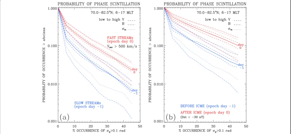
Cumulative probability distribution functions
Figures 6 and 7 show cumulative probability distribution functions (PDFs) for the phase scintillation occurrence in the ‘cusp’ region defined here by latitude range from 70.0°N to 82.5°N and MLT from 0600 to 1800 hours. The PDFs are based on the SPE analysis results shown in Figures 4a and 5a for CIRs and ICMEs, respectively. The curves represent the probabilities that phase scintillation will exceed a given value as plotted on the abscissa.
In Figure 6, the solid lines show overall PDFs for epoch days−1 and 0 (for slow solar wind just before and fast solar wind after the key time) including all solar wind conditions. The overall probability curves for both the slow and fast streams (shown by solid lines) are bracketed by probability curves (broken lines) for scintil-lation data subdivided by corresponding solar wind low and high (below and above median) values ofV, |B|, and σBz. In general, the probabilities are higher for ICMEs
a
b
Figure 4The SPE analysis results based on 108 CIRs.The maps of(a)an average percentage occurrence of phase scintillationσΦexceeding
than for CIRs. As discussed further in the‘Results and dis-cussion’section, the period of slow solar wind before the ar-rival of CIR/HSS is characterized by very low geomagnetic activity and, expectedly, the lowest level of scintillation. It gives the lowest background levels of scintillation occur-rence and thus the lowest probabilities, particularly for the case of low (below median) values of |B| andσBz. Because
ICMEs can arrive when a HSS is active, the mean ‘ back-ground’level of probabilities before the arrival of ICMEs is
expectedly higher. By the same token, the scintillation occurrence (probability) level after an ICME arrival is a superposition of that ‘background’ level and scintillation caused by the ICME interaction with the magnetosphere-ionosphere system. The PDFs shown for low and highV, |B|, andσBzindicate that variability about the average of the
solar wind speed affects the computed probability values the least. The scintillation occurrence (probability) is strongly affected by the variability of the magnetic field.
a
b
Figure 5Same as Figure 4a,b but for the SPE analysis based on 40 ICMEs.
Figure 6The cumulative PDFs in the‘cusp’for days−1 and 0.Probability of the phase scintillation occurrence for(a)slow and fast solar wind on days just before and after CIRs (n= 108) and(b)days just before and after ICMEs (Dst<−30 nT;n= 40). The overall probabilities for each case (solid lines) are bracketed by a pair of curves (broken lines) for data corresponding to low and high (below and above median) values of the mean solar wind velocity,V(dashed lines), magnetic field magnitude, |B| (dash-dot line), and standard deviation of IMFBZcomponent,
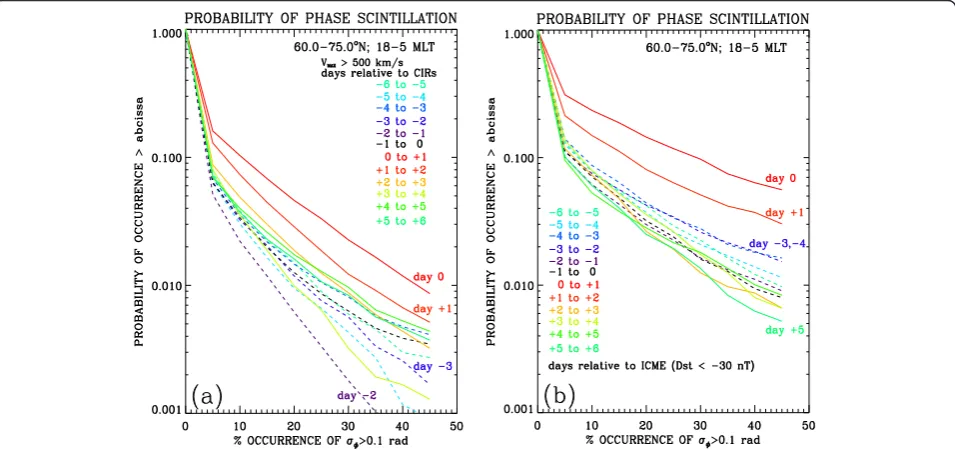
In Figure 7a,b, the overall PDFs are shown from−6 to +6 epoch days stepped by 1-day intervals for HSS/CIRs and ICMEs, respectively. In both cases, the highest probabilities are observed for day 0 (i.e., over 24 h after the key time) but are significantly higher for ICMEs. Although the back-ground levels of occurrences, and thus the PDF values, are higher for the case of ICMEs than for HSS/CIRs; the range of probabilities is larger for the latter. It is noted that the
lowest occurrences (Figures 3a and 4) and the lowest prob-abilities (Figures 7a and 8b) are observed 2 days before HSS/CIR arrivals, i.e., on epoch day−2.
To differentiate between the response in the cusp and auroral zone, Figures 8 and 9 show the cumulative PDFs for the phase scintillation occurrence in the nighttime auroral zone defined here by a latitude range from 60.0°N to 75.0°N and MLT from 1800 to 0600 hours. Clearly, the
Figure 7The cumulative PDFs in the‘cusp’for days−6 to +6.Probability of the phase scintillation occurrence stepped by 1-day intervals before and after(a)CIRs (n= 108) and(b)ICMEs (Dst<−30 nT;n= 40). The line colors correspond to days before and after CIR/ICME as shown in the legend. The days before CIR/ICME are shown in broken lines (from black to blue to cyan); the days after CIR/ICME are shown in solid lines (red to yellow to green).
probabilities are significantly lower as already indicated by lower occurrence rate of phase scintillation in the aur-oral oval as compared with the cusp (Figures 4a and 5a). However, in all instances, both in the cusp and in the aur-oral zone, the highest probability of phase scintillation occurrence is on epoch day 0, i.e., just after the arrival of CIRs or ICMEs. Also, the probabilities are higher for lar-ger values of |B|,σBz, andV. The variability of the
mag-netic field affects the probabilities the most.
Results and discussion
Because of complexity of the solar wind-magnetosphere-ionosphere coupling and the resulting ionospheric ir-regularities, it is generally very difficult or impossible to predict radio scintillation for a given ray path based on physical modeling of the ionospheric structure. Thus, probabilistic forecasting based on statistical results over many years for specific conditions either in solar wind or in the ionosphere appears to be appropriate approach in forecasting scintillation at high latitudes. Since the solar wind disturbances like CIRs and ICMEs are the major causes of geomagnetic and ionospheric distur-bances that result in enhanced scintillation, we applied the forecasting method by McPherron and Siscoe (2004) to forecast phase scintillation occurrence at high latitudes. Initial results (Prikryl et al. 2012) have demonstrated the feasibility of probabilistic forecasting of scintillation in the cusp for a given location of a GPS receiver. In this paper, we use the statistical data from a network of receivers to map the scintillation occurrence as a function of magnetic latitude and MLT. Focusing on specific solar wind events (CIRs and ICMEs), the SPE analysis can provide average
occurrence rate and average number of cycle slips relative to arrival time of CIRs or ICMEs, as a function of magnetic latitude and MLT. Based on these statistical results, one can then construct cumulative PDFs. The PDFs can be specified for a range of magnetic latitudes and MLTs, and also for different solar wind conditions. They can be then used in probabilistic forecasting of scintillation occurrence at high latitudes.
GPS scintillation databases with improved spatial cover-age in latitude/longitude including polar cap and auroral oval, as well as coverage over a complete solar cycle, are needed. The present data cover mostly the last, anomal-ously extended, solar minimum and rise of solar cycle 24, and the majority of ICMEs caused only weak geomagnetic disturbances; none of the ICMEs resulted in a major geo-magnetic storm, e.g., Richardson (2013), which is clearly not representative of periods of high solar activity. In com-parison, strong and recurrent high-speed streams from cor-onal holes remained active during most of the period studied in this paper. The obtained mean probability curves for days before and after CIR arrival are expected to be similar throughout the solar cycle, although they may re-flect the differences between slow and fast solar winds that are likely to be enhanced during the declining phase when the recurrent streams are dominant.
As we have already discussed in the‘Cumulative prob-ability distribution functions’ section, the SPE analysis keyed by the HSS/CIR arrivals resulted in lower back-ground levels of occurrences and probabilities (before epoch day 0), which is partly because of large contribu-tion from years of solar minimum when HSSs regularly occur, while ICMEs are mostly absent. The lowest
scintillation occurrences and lowest probabilities are found for epoch day−2, i.e., 2 days before HSS/CIR arrival. This is consistent with the periods of ‘calm’(Borovsky and Steinberg 2006) during 2 days of slow solar wind just before the major CIR/HSS arrival that is followed by about two ‘stormy’ days of fast solar wind disturbances. The latter solar wind variation is then mirrored by geomagnetic activity (Figure 3a) as well as scintillation and cycle slip occurrence.
MCs are a subset of ICMEs with a smoothly rotating and stronger-than-average magnetic field, as well as low proton temperature (Burlaga et al. 1981). ICMEs associated with MCs are known to be more geoeffective (Huttunen et al.
2005) than non-MC ICMEs. Even small-scale magnetic ropes are found to induce substorm activity (Zhang et al. 2013). Strong ionospheric scintillation was observed during the magnetic cloud-induced geomagnetic storm of April 5 to 7, 2010 (Prikryl et al. 2011b). The scintillation occur-rence during that event increased in the auroral oval in both the northern and southern hemispheres as the MC magnetic field rotated southward. As already discussed in the ‘Methods’ section, we use the MC classification of ICMEs based on the catalogue of ICMEs by Richardson and Cane (2010). Out of 40 ICMEs (Dst <−30 nT) used in the present SPE analysis (Figure 5), 27 cases were classi-fied as MCs indicating all required characteristics of MCs
(l= 2), while 13 cases lacked some or all important char-acteristics of MCs (l= 0 or 1).
Figure 10a,b,c,d shows the PDFs for ‘nightside auroral zone’ (Figure 10a,b) and ‘cusp’ (Figure 10c,d) obtained by the SPE analysis for the subsets of MC (n= 27) and non-MC (n= 13) events. In the‘nightside auroral zone’, the probabilities of scintillation occurrence just after ar-rival are significantly higher for MC events (Figure 10b) compared to the non-MC events (Figure 10a). This is consistent with the finding that MCs are associated with increased substorm activity (Huttunen et al. 2005; Zhang et al. 2013). In the ‘cusp’, while the PDFs just after the arrival of an event (epoch day 0) are very similar for non-MC (Figure 10c) and MC (Figure 10d) events, the ‘background’PDFs before and a few days after the epoch day 0 are lower for the MC subset (Figure 10d). This suggests that, both in the cusp and auroral oval, the differ-ence between the probability of scintillation occurrdiffer-ence just after ICME arrival and probability of scintillation occur-rence before and a few days after the event is higher for the MC events than for the non-MC events.
These results are based on a relatively small statistical sample, and while they represent a proof of concept, a larger statistical sample is needed to further refine the scintillation forecasting method by compiling PDFs sep-arately for different seasons, levels of solar activity, various threshold values ofσΦ, and different magnetic latitudes and local times. Also, it will be important to consider periods of southward and northward IMF since the IMFBZ
compo-nent (in the geocentric solar magnetospheric coordinate system (GSM)) controls the coupling to the magnetosphere and the energy deposition into the ionosphere, which, in turn, affects the ionospheric structure and thus the scintilla-tion level.
As already discussed previously (Prikryl et al. 2012), the feasibility of probabilistic forecasting of scintillation relative to solar wind disturbances will be dependent on accurate prediction of CIR or CME arrivals. Space wea-ther forecasting has benefited from advances in MHD modeling of CMEs and CIRs (Odstrcil et al. 2005; Wu et al. 2011). Multi-spacecraft tracking of CIRs propagation (Williams et al. 2011; Davis et al. 2012) and forecasting propagation and evolution of CMEs in an operational setting (Zheng et al. 2013) are being developed. The viability of probabilistic forecasting of ionospheric scintillation will hinge upon the progress of the solar wind modeling and monitoring efforts to improve space weather forecasting in general.
Conclusions
The SPE analysis is applied to time series of phase scin-tillation and cycle slip occurrence observed by CHAIN from 2008 to 2012. Arrival times of HSS and ICME were used as key times for the SPE analysis. Mapped as a
function of magnetic latitude and magnetic local time, phase scintillation and cycle slips occur predominantly on the dayside in the cusp and in the nightside auroral oval. The scintillation and cycle slips peak on days when HSS or ICME impacts the Earth's magnetosphere. The occurrence of phase scintillation and cycle slips taper off more gradually and reach the mean background levels a few days after the arrival of HSS. In contrast, the occur-rence peaks significantly higher just after the ICME im-pact but drops to background levels 1 or 2 days after the ICME arrivals. The ICMEs of magnetic cloud type result in higher occurrence of scintillation and cycle slips in the nightside auroral oval when compared to the non-magnetic cloud ICMEs. Cumulative probability distribu-tion funcdistribu-tions for the phase scintilladistribu-tion occurrence as a function of epoch day relative to the HSS or ICME ar-rival are obtained for typical cusp and auroral oval loca-tions. The probability distribution functions can also be specified for low and high (below and above median) values of various solar wind plasma parameters. These results can be used to predict occurrence of phase scin-tillation and cycle slip occurrence; however, a larger stat-istical dataset covering at least one solar cycle is needed to develop a probabilistic forecasting method.
Competing interests
The authors declare that they have no competing interests.
Authors' contributions
PP designed this study, analyzed the data, and wrote the manuscript. PTJ conceived of and implemented the CHAIN project and helped in interpretation of the data. SCM contributed to the analysis and interpretation of the GPS data. IGR maintained the archive of the ICMEs and helped in the interpretation of the solar wind data. All authors read and approved the final manuscript.
Acknowledgements
Infrastructure funding for CHAIN was provided by the Canada Foundation for Innovation and the New Brunswick Innovation Foundation. CHAIN operation is conducted in collaboration with the Canadian Space Agency (CSA). The solar wind data were obtained from Goddard Space Flight Center Space Physics Data Facility OMNIWeb (http://omniweb.gsfc.nasa.gov/). This work was supported by the Public Safety Geosciences program of the Natural Resources Canada, Earth Sciences Sector (NRCan ESS Contribution Number 20130496).
Author details 1
Geomagnetic Laboratory, Natural Resources Canada, 2617 Anderson Rd, Ottawa, ON K1A 0E7, Canada.2Physics Department, University of New
Brunswick, Fredericton, NB E3B 5A3, Canada.3Department of Physics and Astronomy, University of Calgary, Calgary, AB T2N 1N4, Canada.4CRESST and
Department of Astronomy, University of Maryland, College Park, MD 20742, USA.5NASA Goddard Space Flight Center, Greenbelt, MD 20771, USA.
Received: 12 March 2014 Accepted: 12 May 2014 Published: 30 June 2014
References
Aarons J (1982) Global morphology of ionospheric scintillations. Proc IEE 70 (4):360–378
Aarons J (1997) Global positioning system phase fluctuations at auroral latitudes. J Geophys Res 102(A8):17219–17231, doi:10.1029/97JA01118
Basu S, MacKenzie EM, Basu S, Costa E, Fougere PF, Carlson HC Jr, Whitney HE (1987) 250 MHz/GHz scintillation parameters in the equatorial, polar, and auroral environments. IEEE J Select Areas Commun SAC-2(2):102–115 Basu S, Basu S, Sojka JJ, Schunk RW, MacKenzie E (1995) Macroscale modeling
and mesoscale observations of plasma density structures in the polar cap. Geophys Res Lett 22(8):881–884, doi:10.1029/95GL00467
Basu S, Weber EJ, Bullett TW, Keskinen MJ, MacKenzie E, Doherty P, Sheehan R, Kuenzler H, Ning P, Bongiolatti J (1998) Characteristics of plasma structuring in the cusp/cleft region at Svalbard. Radio Sci 33(6):1885–1899, doi:10.1029/ 98RS01597
Borovsky JE, Steinberg JT (2006) The“calm before the storm”in CIR/ magnetosphere interactions: occurrence statistics, solar wind statistics, and magnetospheric preconditioning. J Geophys Res 111:A07S10, doi:10.1029/ 2005JA011397
Burlaga L, Sittler E, Mariani F, Schwenn R (1981) Magnetic loop behind an interplanetary shock - Voyager, Helios, and IMP 8 observations. J Geophys Res 86:6673–6684
Conker RS, El Arini MB, Hegarty CJ, Hsiao T (2003) Modeling the effects of ionospheric scintillation on GPS/satellite-based augmentation system availability. Radio Sci 38(1):1001, doi:10.1029/2000RS002604
Davis CJ, Davies JA, Owens MJ, Lockwood M (2012) Predicting the arrival of high-speed solar wind streams at Earth using the STEREO Heliospheric Imagers. Space Weather 10:S02003, doi:10.1029/2011SW000737 Feldstein YI, Starkov GV (1967) Dynamics of auroral belt and polar geomagnetic
disturbances. Planet Space Sci 15:209–230
Holzworth RH, Meng C-I (1975) Mathematical representation of the auroral oval. Geophys Res Lett 2(9):377–380
Horvath I, Crozier S (2007) Software developed for obtaining GPS-derived total electron content values. Radio Sci 42:RS2002, doi:10.1029/2006RS003452 Huttunen KEJ, Schwenn R, Bothmer V, Koskinen HEJ (2005) Properties and
geoeffectiveness of magnetic clouds in the rising, maximum and early declining phases of solar cycle 23. Ann Geophys 23:625–641, doi:10.5194/ angeo-23-625-2005
Jayachandran PT, Langley RB, MacDougall JW, Mushini SC, Pokhotelov D, Hamza AM, Mann IR, Milling DK, Kale ZC, Chadwick R, Kelly T, Danskin DW, Carrano CS (2009) Canadian High Arctic Ionospheric Network (CHAIN). Radio Sci 44: RS0A03, doi:10.1029/2008RS004046 (printed 45(1), 2010)
Jiao Y, Morton YT, Taylor S, Pelgrum W (2013) Characterization of high-latitude ionospheric scintillation of GPS signals. Radio Sci 48:698–708, doi:10.1002/ 2013RS005259
Li G, Ning B, Ren Z, Hu L (2010) Statistics of GPS ionospheric scintillation and irregularities over polar regions at solar minimum. GPS Solut 14:331–341, doi:10.1007/s10291-009-0156-x
Kavanagh AJ, Honary F, Donovan EF, Ulich T, Denton MH (2012) Key features of >30 keV electron precipitation during high speed solar wind streams: a superposed epoch analysis. J Geophys Res 117:A00L09, doi:10.1029/ 2011JA017320
McPherron RL, Siscoe G (2004) Probabilistic forecasting of geomagnetic indices using solar wind air mass analysis. Space Weather 2:S01001, doi:10.1029/ 2003SW000003
McPherron RL, Weygand J (2006) The solar wind and geomagnetic activity as a function of time relative to corotating interaction regions. In: Tsurutani B, McPherron RL, Gonzalez W, Lu G, Sobral JHA, Gopalswamy N (eds) Recurrent magnetic storms: corotating solar wind streams. AGU Monograph. AGU, Washington, D.C, pp 125–137, 167
Odstrcil D, Pizzo VJ, Arge CN (2005) Propagation of the 12 May 1997 interplanetary coronal mass ejection in evolving solar wind structures. J Geophys Res 110:A02106, doi;10.1029/2004JA010745
Osherovich VA, Fainberg J, Stone RG (1999) Solar wind quasi-invariant as a new index of solar activity. Geophys Res Lett 26(16):2597–2600
Prikryl P, Jayachandran PT, Mushini SC, Chadwick R (2011a) Climatology of GPS phase scintillation and HF radar backscatter for the high-latitude ionosphere under solar minimum conditions. Ann Geophys 29:377–392, doi:10.5194/ angeo-29-377-2011
Prikryl P, Spogli L, Jayachandran PT, Kinrade J, Mitchell CN, Ning B, Li G, Cilliers PJ, Terkildsen M, Danskin DW, Spanswick E, Donovan E, Weatherwax AT, Bristow WA, Alfonsi L, De Franceschi G, Romano V, Ngwira CM, Opperman BDL (2011b) Interhemispheric comparison of GPS phase scintillation at high latitudes during the magnetic-cloud-induced geomagnetic storm of 5–7 April 2010. Ann Geophys 29:2287–2304, doi:10.5194/angeo-29-2287-2011
Prikryl P, Jayachandran PT, Mushini SC, Richardson IG (2012) Toward the probabilistic forecasting of high-latitude GPS phase scintillation. Space Weather 10:S08005, doi:10.1029/2012SW000800
Prikryl P, Ghoddousi-Fard R, Kunduri BSR, Thomas EG, Coster AJ, Jayachandran PT, Spanswick E, Danskin DW (2013a) GPS phase scintillation and proxy index at high latitudes during a moderate geomagnetic storm. Ann Geophys 31:805–816, doi:10.5194/angeo-31-805-2013
Prikryl P, Sreeja PV, Aquino M, Jayachandran PT (2013b) Probabilistic forecasting of ionospheric scintillation and GNSS receiver signal tracking performance at high latitudes. Spec Issue Ann Geophysics 56(2):R0222, doi:10.4401/ag-6219 Richardson IG (2013) Geomagnetic activity during the rising phase of solar cycle
24. J Space Weather Space Climate 3:A08, doi:10.1051/swsc/2013031 Richardson IG, Cane HV (2010) Near-earth interplanetary coronal mass ejections
during solar cycle 23 (1996–2009): catalog and summary of properties. Solar Phys 264(1):189–237, doi:10.1007/s11207-010-9568-6
Spogli L, Alfonsi L, De Franceschi G, Romano V, Aquino MHO, Dodson A (2009) Climatology of GPS ionospheric scintillations over high and mid-latitude European regions. Ann Geophys 27:3429–3437
Sreeja V, Aquino M, Elmas ZG (2011) Impact of ionospheric scintillation on GNSS receiver tracking performance over Latin America: introducing the concept of tracking jitter variance maps. Space Weather 9:S10002, doi:10.1029/ 2011SW000707
van Dierendonck AJ, Arbesser-Rastburg B (2004) Measuring ionospheric scintillation in the equatorial region over Africa, including measurements from SBAS geostationary satellite signals. In: Proceedings of the 17th International Technical Meeting of the Satellite Division of The Institute of Navigation (ION GNSS 2004). The Institute of Navigation, Long Beach, CA, pp 316–324
Williams AO, Edberg NJT, Milan SE, Lester M, Fränz M, Davies JA (2011) Tracking corotating interaction regions from the Sun through to the orbit of Mars using ACE, MEX, VEX, and STEREO. J Geophys Res 116:A08103, doi:10.1029/ 2010JA015719
Wu C-C, Dryer M, Wu ST, Wood BE, Fry CD, Liou K, Plunkett S (2011) Global three-dimensional simulation of the interplanetary evolution of the observed geoeffective coronal mass ejection during the epoch 1–4 August 2010. J Geophys Res 116:A12103, doi:10.1029/2011JA016947
Zhang X-Y, Moldwin MB, Cartwright M (2013) The geo-effectiveness of interplanetary small-scale magnetic fluxropes. J Atmos Solar-Terr Phys 95–96:1–14
Zheng Y, Macneice P, Odstrcil D, Mays ML, Rastaetter L, Pulkkinen A, Taktakishvili A, Hesse M, Kuznetsova MM, Lee H, Chulaki A (2013) Forecasting propagation and evolution of CMEs in an operational setting: what has been learned. Space Weather 11:557–574, doi:10.1002/swe.20096
doi:10.1186/1880-5981-66-62
Cite this article as:Prikrylet al.:High-latitude GPS phase scintillation and cycle slips during high-speed solar wind streams and interplanetary coronal mass ejections: a superposed epoch analysis.Earth, Planets and Space 201466:62.
Submit your manuscript to a
journal and benefi t from:
7 Convenient online submission
7 Rigorous peer review
7 Immediate publication on acceptance
7 Open access: articles freely available online
7 High visibility within the fi eld
7 Retaining the copyright to your article