JHS, Vol. 4, Issue 1

(1)

(2)

SUMMER 2018, Vol 4, Issue 1, JOURNAL OF HYDRAULIC STRUCTURES

Journal of Hydraulic Structures

Department of Civil Engineering

Faculty of Engineering

Shahid Chamran University of Ahvaz

In the name

of GOD

(3)

HYDRAULIC

STRUCTURES

SHAHID CHAMRAN UNIVERSITY OF AHVAZ Manager: Prof. Hamid R. Ghafouri

Editor-in-chief: Dr. Ali Haghighi

Editorial coordinator:Dr. Seyed Mohammad Ashrafi Department of Civil Engineering, Faculty of

Engineering, Shahid Chamran University of Ahvaz, Ahvaz, Iran.

Members

Prof. Hossein M. V.Samani

Civil Engineering Department, Shahid Chamran University of Ahvaz, Ahvaz, Iran

Prof. Hamid R. Ghafouri

Dr. Ali Haghighi

Prof. Mahmood S. Bajestan

Hydraulic Structures Department, Shahid Chamran University of Ahvaz, Ahvaz, Iran

Prof. Saeed R. S. Yazdi

Civil Engineering Department, K.N.Toosi University of Technology, Tehran, Iran

Dr. Mohammad S. Pakbaz

Dr. Arash Adib

Civil Engeering Department, Shahid Chamran University of Ahvaz, Ahvaz, Iran

Dr. Mojtaba Labibzadeh

Prof. Helena M. Ramos

Instituto Superior Técnico (IST), University of Lisbon

Dr. S. Mohammad Ashrafi

Dr. S. Abbas Haghshenas

Institute of Geophysics, University of Tehran | UT, Tehran, Iran

Dr. Mohammad Zounemat-Kermani

Department of Water Engineering, Shahid Bahonar University of Kerman, Kerman, Iran

Dr. Taher Rajaee

Civil Engineering Department, University of Qom, Qom, Iran

Dr. Mohammad Vaghefi

Civil Engineering Department, Faculty of Engineering, Persian Gulf University, Bushehr, Iran

Dr. A. A. Telvari

Soil Conservation and Watershed Management Research Institute; Department of Civil Engineering, Islamic Azad University, Ahvaz branch, Ahvaz, Iran

I. In the name of God

II. Table of Contents

III. Aims and Scope

01 Development of a Direct Explicit Equation

for Hydraulic Design of Semi-elliptical

Channels

H. Nikroy Motlagh; Hossein M.V. Samani; H. Hassanpour Darvishi

08 An Alternating Direction Implicit Method for

Modeling of Fluid Flow

I. Saeedpanah; A. Adib

19 Wave Evolution in Water Bodies using

Turbulent MPS Simulation

H. Imanian; M. Kolahdoozan; A.R. Zarrati

36 Ocean Currents Modeling along the Iranian

Coastline of the Oman Sea and the

Northern Indian Ocean

M. Jedari Attari; S.A. Haghshenas; A. Bakhtiari; M.H. Nemati

55 Study of Streamlines under the Influence of

Displacement of Submerged Vanes in

Channel Width, and at the Upstream Area of

a Cylindrical Bridge Pier in a 180 Degree

Sharp Bend

C.A. Chooplou; M. Vaghefi; S.H. Meraji

75 Frequency domain analysis of transient flow

in pipelines; application of the genetic

programming to reduce the linearization

errors

(4)

Aims and Scope

Hydraulic Structure Journal is an interdisciplinary journal which publishes high-quality peer-reviewed articles addressing the latest developments and applied methods in construction, maintenance, management, and operation policy of Hydraulic Structures.

The Journal aims at providing an efficient route to fast-track publication, within 10-12 weeks after manuscript submission. Manuscripts will be considered for publication in the following categories: research articles, technical notes, case reports and discussions.

The general areas covered by the Journal include:

 Technical and methodological advances in application, design/selection, production, modification of construction materials

 Advances in numerical and analytical methods

 Hydro informatics and soft computing

 Hydraulic aspects of hydraulic structures

 Applied surface and subsurface hydrology and hydrometeorology

 Forecasting approaches in water resources engineering

 Economic and social aspects of hydraulic structures

 Uncertainty analysis and risk management in hydraulics and water resources engineering

 Application of Nanotechnology in Hydraulic Structures

 Geotechnics of Hydraulic Structures

 Damage detection techniques

The following might be considered as hydraulic structures:

 Dams and associated structures

 River and Watershed Structures

 Offshore and Onshore Structures

 Irrigation and Drainage Channel Networks

 Bridges

 Water Storage and Conveyance Structures

 Pipelines and Pump Stations

 Sewerage Systems

 Water and Wastewater Treatment Plants

 Historical Water Structures

General Information

Title: Journal of Hydraulic Structures

Subject: Hydraulics and water resources engineering Coverage area: International

Journal Type: Scientific and technical

License Holder: Shahid Chamran University of Ahvaz Editor-in-Chief: Dr. Ali Haghighi

Manager: Prof. Hamid R. Ghafouri

Editorial coordinator: Dr. Seyed Mohammad Ashrafi

Language Editors: Majid SadollahKhani Soroosh Kamali

Address: Department of Civil Engineering, Faculty of Engineering, Shahid Chamran University of Ahvaz

Phone #: +986133330011-19 (5610 & 5603)

(5)

SUMMER 2018, Vol 4, Issue 1, JOURNAL OF HYDRAULIC STRUCTURES Shahid Chamran University of Ahvaz

Journal of Hydraulic Structures

J. Hydraul. Struct., 2018; 4(1):1-7 DOI: 10.22055/JHS.2018.24972.1066

Development of a Direct Explicit Equation for Hydraulic

Design of Semi-elliptical Channels

Hossein Nikroy Motlagh1 Hossein M. V. Samani2 Hossein Hassanpour Darvishi3

Abstract

One of the common concrete channels in irrigation networks is the semielliptical prefabricated channels. Manning formula is usually used to design these channels. The cross-sectional area and the wetted perimeter are required to be calculated in Manning formula. There are no analytical solutions to directly compute these parameters. Thus, numerical integration methods are inevitably used. In this paper, a wide number of various semielliptical channels are regarded and their cross-sectional areas and wetted perimeters for different depths were computed numerically to produce databases for three-dimensional curve fitting. Direct relationships for the cross-sectional area and the wetted perimeter in terms of the channels size and the hydraulic parameters were developed. These relationships were used in the design of the semielliptical concrete channels and the results were compared with the numerical ones. The results were quite close to each other.

Keywords: semielliptical, Manning formula, Numerical method, correlation coefficient

Received: 11 February 2018; Accepted: 10 April 2018

1. Introduction

Now a day, prefabricated concrete channels are widely used in irrigation networks. These channels are constructed in various shapes. This includes traditional sections such as trapezoidal ones [1, 2, 3, 4] and parabolic sections [5, 6, 7]. One of the other channel sections used is the elliptic sides with horizontal bottoms [8]. The semielliptical concrete channels have been

1_{Graduate student, Water Resources Engineering Department, Faculty of Engineering, Shahr Qods}

Islamic Azad University, Shahr Qods, Tehran.

2_{Professor, Water Resources Engineering Department, Faculty of Engineering, Shahr Qods Islamic Azad}

University, Shahr Qods, Tehran. (Corresponding author)

3_{Associated Professor, Water Resources Engineering Department, Faculty of Engineering, Shahr Qods}

(6)

recently widely utilized in irrigation projects. They have the advantages of reducing of the constructional cost and land acquisition, reducing evaporation by having smaller water surface widths, reducing sedimentation and they can be constructed fast [9, 10, 11, 12]. There are no explicit direct solutions for the semielliptical cross sections and the wetted perimeters to be used in Manning formula. Vatankhah [12], used a numerical method to calculate the integrals of the cross-section and the wetted perimeter.

In this research, explicit direct relationships for the cross-sectional area and the wetted perimeter of the semielliptical channels are found by using three-dimensional regression analysis. Then, they were used in Manning formula for design purposes.

2. Design Method

Manning formula is used for the design of the semielliptical channels as follows:

2 / 1 0 3 / 2

1 AS

R

n

Q



(1)

Where:

Q= Flow discharge

n

= Manning coefficient

R= Hydraulic radius which is equal to the ratio of the flow cross-sectional area, A, to the wetted perimeter, P

0

S

= Channel bed slope

The flow discharge, Manning coefficient, and the channel bed slope are known. There are many prefabricated concrete semielliptical channels available in the market. The economic optimum design of the semielliptical channel should have the capacity to carry the flow with a limited freeboard. A computer program is developed in this regard in which all the prefabricated available channel sizes are used in the calculation and then the smallest size that is able to pass the flow properly is chosen. The integrals of the cross-sectional areas and the wetted perimeters are calculated by using the trapezoidal rule.

3. Calculation of Flow Cross Sectional Area and Wetted-Perimeter

Figure 1 depicts a typical semielliptical cross-section in which a and b are the horizontal and vertical radii of the ellipse, respectively. The cross-section is symmetrical with respect to the y-axis. Hence, it is possible to calculate half of the total cross section and then multiplies that by 2 to obtain the total cross-sectional area. The half cross-section is divided into several elements as shown in the figure. Each element is assumed to be trapezoidal. The coordinates of the intersections of the vertical lines of the elements with the elliptical curve of the channel wall can be determined by the equation:

1 ) (

) (

2 2 0 2

2

0   



b y y a

x x

(2)

(7)

Figure 1. Flow Cross Sectional Area in the Semi-elliptical Channel

The wetted perimeter of each element depicted in Figure 1 can be calculated by the following equation:

2 1 2

1 2

2

)

(

)

(

)

(

)

(

i i i i

i

x

y

x

y

L



















_ _ (3)

In which

(

x

_i

,

y

_i

)

and

(

x

_i_₁

,

y

_i_₁

)

are the coordinates of two sequential points of the ellipse shown in Figure 1. The summation of



L

_is results in half of the total wetted perimeter. As an example, semielliptical prefabricated concrete types are considered for the design of a channel to carry out 500 L/s and the bed slope is 0.0005. Manning coefficient is regarded as 0.015. The results of the developed computer program are introduced in Table 1.

Table1. Semielliptical channel types for the given example

Type Depth (cm) b(cm) a(cm) n Q(L/s) Qcalc(L/s) Bed Slope

70 26.4 33.4 27.7 0.015 500 15.1609 0.0005

80 28.7 35.7 29.6 0.015 500 18.6132 0.0005

100 32.9 39.9 32.9 0.015 500 25.8852 0.0005

120 36.7 43.7 36 0.015 500 33.9412 0.0005

135 39.4 46.4 38.1 0.015 500 40.3424 0.0005

150 41.9 48.9 40 0.015 500 46.8109 0.0005

180 44.6 51.6 45.4 0.015 500 61.1335 0.0005

200 45.6 52.6 49.4 0.015 500 71.2627 0.0005

230 48.8 55.8 53.5 0.015 500 87.2413 0.0005

250 48.9 55.9 58 0.015 500 98.5231 0.0005

280 50.5 57.5 63 0.015 500 115.764 0.0005

(8)

350 53.9 60.9 74.6 0.015 500 160.501 0.0005

400 55.6 62.6 82.8 0.015 500 193.766 0.0005

450 56.1 63.1 92.2 0.015 500 227.925 0.0005

520 56.5 63.5 105.6 0.015 500 277.212 0.0005

600 58.2 65.2 118.7 0.015 500 337.818 0.0005

700 62.8 69.8 135.6 0.015 500 447.656 0.0005

800 64.62604954 74.4 144.7 0.015 500 500 0.0005 900 62.74162577 78.7 153.4 0.015 500 500 0.0005

1000 61.23847894 82.8 161.6 0.015 500 500 0.0005

The first column of Table 1 represents the channel type and the calculated flow depths are given in the second column. The third and fourth columns represent the vertical and horizontal radii, respectively. The seventh column represents the calculated flow corresponds to the channel size types. The results show that channel types 70 to 700 are too small to pass the given flow and types 800, 900, and 1000 are able to pass the flow. It is clear that type 800 is the economical one which should be regarded as a final design.

4. Explicit Relationships for the Flow Cross Sectional Area and the Wetted

Perimeter

In order to develop explicit direct relationships for the flow cross-sectional area and the wetted perimeter, a large number of condition combinations of semielliptical channels with various hydraulic conditions are considered. The developed computer program is applied to all these combinations similar to that which is shown in Table 1. Based on the obtained results the dimensionless flow cross-sectional area 𝐴⁄_𝑎𝑏 is regarded as a function of the dimensionless

variables 𝑦⁄ , 𝑦 𝑏_𝑎 ⁄ and the least squares method was used to obtain the best fitted function. This

task was done by the Table-curve 3D software. The results indicated that 𝐴⁄_𝑎𝑏 is only a function

of 𝑦 𝑏⁄ and the best-fitted function is obtained as:

) / ( 46526 . 1 ) / ( 111776 . 0 552486 .

0 y b2 Ln y b

e

ab

A

_

 

(4)

The correlation coefficient for the above function is calculated as r2 0.99999994. Similarly, the dimensionless wetted perimeter 𝐿

√𝑎2_{+ 𝑏}2

⁄ is considered as a function of the

dimensionless variables 𝑦⁄ , 𝑦 𝑏_𝑎 ⁄ and the best-fitted function is obtained as:

3992385 .

1 / 2257358 .

3 /

413705 .

0

2

2_  _y _a  y b

b a

L

(5)

The correlation coefficient for the function given in Equation (5) is calculated as 99999994

. 0

2 

r .

(9)

) 6 ( 3992385 . 1 / 2257358 . 3 / 413705 . 0 1 0 ) / ( 46526 . 1 ) / ( 111776 . 0 552486 . 0 3 / 2 2 2 ) / ( 46526 . 1 ) / ( 111776 . 0 552486 . 0 2 2 S abe b y a y b a abe n

Q yb Lnyb

b y Ln b y                              

The developed equation (6) can be used simply for the design of semielliptical channels.

5. Evaluation of the Developed Equation

Various semielliptical channels with different slopes are considered and the flow discharges are calculated by two methods, the developed equation [Equation (6)] and the numerical trapezoidal method. The results are given in Table 2. Column 7 represents the difference percent between the developed and numerical methods. It is noted that the differences are very small which proves that the developed equation has the desired accuracy.

Table2. Percent of differences Between the Developed Equation and The Numerical Method

Depth (cm) a b Bed Slope S n Q Eq.(6) Q(Numerical) Error %

46.23724 0.315 0.575 0.0005 0.015 99.9 99.99 0.10001

43.25029 0.345 0.593 0.0005 0.015 99.59 99.99 0.414032

51.95147 0.461 0.631 0.0005 0.015 200.17 200 0.08504

46.93797 0.528 0.635 0.0005 0.015 199.86 200 0.067927

54.36399 0.5935 0.652 0.0005 0.015 299.2 300 0.268229

58.88418 0.678 0.698 0.0005 0.015 398.07 400.00 0.484581

64.62605 0.7235 0.744 0.0005 0.015 497.41 500.00 0.520581

62.74163 0.767 0.787 0.0005 0.015 497.97 500 0.406979

69.53065 0.767 0.787 0.0005 0.015 596.76 600 0.542812

67.69017 0.808 0.828 0.0005 0.015 597.29 600 0.454458

46.67753 0.29 0.559 0.0006 0.015 100.05 100 0.05304

43.82707 0.315 0.575 0.0006 0.015 99.65 100 0.350047

53.65199 0.414 0.626 0.0006 0.015 200.52 200 0.258765

49.30414 0.461 0.631 0.0006 0.015 199.98 200 0.01005

56.09775 0.528 0.635 0.0006 0.015 300.01 300 0.003339

51.65093 0.5935 0.652 0.0006 0.015 299.32 300 0.22821

55.95632 0.678 0.698 0.0006 0.015 398.38 400 0.407195

61.38002 0.7235 0.744 0.0006 0.015 497.72 500 0.457451

66.01671 0.767 0.787 0.0006 0.015 597.08 600 0.488993

70.12686 0.808 0.828 0.0006 0.015 696.47 700 0.506404

75.71512 0.808 0.828 0.0006 0.015 795.54 800 0.560142

6. Summary and Conclusions

(10)

and the wetted perimeters are calculated by using the trapezoidal numerical integration method. A large number of the database include the flow discharges against the channel characteristics were provided by the developed computer program. The database was converted to dimensionless parameters for the cross-sectional area and the wetted perimeter versus other dimensionless hydraulic parameters and then the Table-curve 3D software was utilized to obtain the best functions which fit the data using the least square method. As a result, explicit direct equations were obtained whose correlation coefficients are equal to almost unity which indicate that the fitted functions have desired accuracies. The accuracy of the developed final equation of the Manning formula was tested by comparing its results with those obtained by the numerical integration method. The results indicate close agreement with each other which shows that the developed explicit direct Manning equation can be used for the purpose of semielliptical channel design with a proper accuracy.

7. References

1. Guo, C. and Hughes, W. (1984). “Optimal channel cross-section with freeboard.” Journal of Irrigation and Drainage Engineering, Vol. 110, No. 3, pp. 304-314, DOI:

10.1061/(ASCE)0733-9437(1984)110:3(304).

2. Frochlich, D. C. (1994). “Width and depth constrained best trapezoidal section.“ Journal of Irrigation and Drainage Engineering, Vol. 120, No. 4, pp. 828-835, DOI: 10.1061/(ASCE) 0733-9437 (1994)120:4(828).

3. Jain, A., Bhattachariya, R. K. and Sanaga, S. (2004). “Optimal design of composite channels using a genetic algorithm. “Journal of Irrigation and Drainage Engineering, Vol. 130, No. 4, pp. 286-295. DOI: 10.1061/(ASCE)0733-9437(2004)130:4(286).

4. Bhattachariya, R. K., and Satish, M. G. (2007). “Optimal design of a stable trapezoidal cross section using hybrid optimization technique.” Journal of Irrigation and Drainage

Engineering, Vol. 133, No. 4, pp. 323-329, DOI: 10.1061/(ASCE) 0733-9437 (2007) 133:4(323).

5. Longanathan, G. V. (1991). “Optimal design of parabolic canals.” Journal of Irrigation and Drainage Engineering, Vol. 1117, No. 5, pp. 716-735, DOI: 10.1061/(ASCE) 0733-9437 (1991)117:5(716).

6. Chahar, B. R. (2005). “Optimal design of parabolic canal section.” Journal of Irrigation and Drainage Engineering, Vol. 131, No. 6, pp. 546-554, DOI: 10.1061/(ASCE) 0733-9437 (2005)131:6(546).

7. Aksoy, B. and Altan-Sakarya, A. (2006). “Optimal lined channelDesign.” Canadian Journal of Civil Engineering, Vol. 33, No. 5, pp. 535-545, DOI: 10.1139/106-008.

(11)

11. Dey, S. and Papanicolaou, A. (2008). “Sediment threshold under streamflow: A state-of-the- art review.“ Korean Journal of Civil Engineering, Vol. 12, No. 1, pp. 45-60, DOI:

10.1007/s12205-015-0494-x.

(12)

An alternating direction implicit method for modeling of fluid

flow

Iraj Saeedpanah1 Arash Adib2

Abstract

This research includes of the numerical modeling of fluids in two-dimensional cavity. The cavity flow is an important theoretical problem. In this research, modeling was carried out based on an alternating direction implicit via Vorticity-Stream function formulation. It evaluates different Reynolds numbers and grid sizes. Therefore, for the flow field analysis and prove of the ability of the scheme, the numerical solution was carried out for different values of the Reynolds numbers. Also, the behavior of the vortex flow in cavity was predicted. This research compares results of applied numerical model with the results of Chia et al. [1] and Chen & Pletcher [2]. Comparing the results with those of the benchmarks show that alternating direction implicit is an effective and suitable formulation for the solution of the Navier–Stokes equations.

Keywords: Alternating direction implicit, Unsteady 2-D incompressible N-S equation, Two-dimensional, Cavity, Vortex flow

Received: 26 December 2017; Accepted: 22 April 2018

1. Introduction

Developing numerical methods for solving the Navier-Stokes equations (NSE) has its own challenges and difficulties. Also, the development of numerical methods to simulate fluid flows with applications has been a research area of great progress over the past half-century. The very common schemes used in computational fluid dynamics could be divided into three categories as: finite difference methods (FDM), finite element methods (FEM) and finite volume methods (FVM). Investigation about hydraulic structures is an interesting subject. Therefore, there are many studies which examine the hydraulic structures in different geometries. Driesen et al. [3] analyzed the flow pattern in a cavity. This problem thus is a good test for experimental flow

1_{Assistant Professor, Department of Civil Engineering, Faculty of Engineering, University of Zanjan,}

Zanjan, Iran. (*Corresponding author, [email protected])

2_{Associate Professor, Department of Civil Engineering, Shahid Chamran University of Ahvaz, Ahvaz,}

(13)

research [4–7]. Gurcan [8] researched about the effect of the Reynolds number on streamline cavity with free surfaces. An incompressible flow behavior inside the different triangular cavities is also presented in [7]. In addition, other researchers such as Agarwal [10], Ghia et al. [1], Chen and Pletcher [2] have studied about the numerical solution of NSE. The most recent works carried out in this regard are those by Ghia & Shin and Chen. They have analyzed the flow field in a cavity for the examination of their solution with different Reynolds numbers. Consequently, in this research, also, flow field in a cavity was taken as the case study, so that, the results of the simulations could be compared with the results of the simulations done by other researchers. According to Anderson et al. [11], the cavity is an excellent test for the solution of NSE for an incompressible fluid flow. This case of flow is important for inspection of the results from the view point of the ability of the scheme to predict complex of the flow fields. Moreover, in the case of flow in a cavity, vortex flow in a bounded geometry is created. Simulation of such a flow is of vital importance from the view point of applications of this type of flow. In this research, analysis of flow field in a cavity with Reynolds number of 100, 400, 1000 and 2000 was carried out by solving NSE.

2. Methodology

The problem considers incompressible flow in a cavity with an upper lid moving with a velocity U as shown in Figure 1.

Figure 1. Schematic of the cavity flow

The general non-dimensional, non conservative form of NSE:

(14)

Application of certain mathematics operations on the Eqs, (1), (2) and (3) for the purpose of obtaining a Vorticity–Stream function formulation, the above equations are given in the following form as

                         2 2 2 2 Re 1 y x y v x u

t (2)













2 2 2 2

y

x



(3)

which are of parabolic and elliptic type, respectively.

An important advantage of this formulation is that pressure is not appeared in the above equations explicitly. So, the Vorticity–Stream function formulation does not contain the pressure term. x v y u      





,



(4)

                                      

 ₂ 2

2 2 2 2 2 2 2 2 2 y x y x y p x

p



(5)

Using numerical formulation of Vorticity-Stream function and employing the ADI scheme and Eq. (11), the velocity field is computed.

2.1. Discretization of vorticity equation

With regard to the fact that Eq. (4) is of parabolic type, this equation is discretized using the ADI scheme resulting in the efficient use of the nodes from the entire boundary. This provides high accuracy and more physical adaptation of the solution. More over with this scheme, three diagonal sets of equations are solved instead of five diagonal sets of equations. There is possibility of selection of better space and time steps and unconditional stability exists. Solution of ADI formulation gives the two following equations which are solved successively:

2 1 , , 1 , 2 , 1 , , 1 1 , 1 , , , 1 , 1 , , ,

)

(

2 Re

1 )

(

2 Re

1

2

2 /

)

(

2 1 2 1 2 1 2 1 2 1 2 1

y

x

y

V

x

U

t

n j i n j i n j i n j i n j i n j i n j i n j i n j i n j i n j i n j i n j i n j i

























































              (6-a) 2 1 1 , 1 , 1 1 , 2 , 1 , , 1 1 1 , 1 1 , , , 1 , 1 , , 1 ,

)

(

2 Re

1 )

(

2 Re

1

2

2 /

)

(

2 1 2 1 2 1 2 1 2 1 2 1 2 1 2 1

y

x

y

V

x

U

t

n j i n j i n j i n j i n j i n j i n j i n j i n j i n j i n j i n j i n j i n j i

























































                      (6-b)

(15)





n _x

j i x x n j i x n j i x

x

d

C

d

D

C

















_





















_



     2 1 2 1 2 1 , 1 , , 1

2

1

2

1

2

1

2

1

(7-a)





y

n j i y y n j i y n j i y

y

d

C

d

D

C

















_





















_



   

 ,11

1 , 1 1 ,

2

1

2

1

2

1

2

1

(7-b)

where the Courant and diffusion numbers are defined as

2 2 ) ( Re 1 , ) ( Re 1 , y t d x t d y t v C x t u C y x y x            

The right hand sides of Eq. (7) are defined respectively as





n

j i y y n j i y n j i y y

x C d d C d

D , 1 , , 1

2 1 2 1 1 2 1 2 1        _ _            _

 (8-a)





12 12

2 1 , 1 , , 1 2 1 2 1 1 2 1 2 1           _ _            _  n j i x x n j i x n j i x x

y C d d C d

D (8-b)

The values of u and v used in Eq. (7) could be used at time n or n+1/2. If the later time is taken, the stream function equation should be solved at time n+1/2, for which larger computation time will be utilized. Simplification of the above equations leads to

y n j i y n j i y n j i y x n j i x n j i x n j i x

D

C

B

A

D

C

B

A

























          2 1 2 1 2 1 2 1 2 1 2 1 1 , , 1 , , 1 , , 1 (9) in which

)

2

1 (

2

1

1 )

2

1 (

2

1 )

2

1 (

2

1

1 )

2

1 (

2

1

y y y y y y y y x x x x x x x x

d

C

d

B

d

C

A

d

C

d

B

d

C

A





























(10)

2.2. Discretization of stream function equation

Regarding that the stream function Eq. (3) is of elliptic type, the Guass Seidal point to point method is employed for solving this equation as

 

2





1 1 2 1

, 2 , 1, 1, , 1 , 1

1

2(1 )

k k k k k k

i j x i j i j i j i j i j



 





          _       _

(16)

in which y x   



(12)

Computation begins with solving the vorticity Eq. (6). Then, the vorticity in Eq. (11) is given a new value and the stream function equation is solved for . This process is repeated until the final convergent solution is achieved. After  computation, the velocity components are computed using Eq. (4).

x

2 ψ

ψ

v

y

2 ψ

ψ

u

j 1, -i j 1, i j i, 1 -j i, 1 j i, j i,













  (13)

2.3. Discretization of poison equation

Computing the final flow field, in order to obtain pressure field, the poison Eq. (5) is discretized as follows;























2 2 2 2 2 2 2

)

(

)

(

)

(

2 y

x

y

x

p



(14)

This equation could be rewritten as

S P 2 (15) In which                                    2 2 2 2 2 2 2 y x y x

S



(16)

Therefore, we would have

                                                   2 1 , 1 1 , 1 1 , 1 1 , 1 2 1 , , 1 , 2 , 1 , , 1 , 4 ) ( 2 ) ( 2 2 y x y x S j i j i j i j i j i j i j i j i j i j i j i



(17)

Now, having Si,j and using the point by point Guass-Seidal elimination to discretize Eq. (15),

pressure at all points of the flow domain is computed by







1



1 , 1 , 2 1 , 1 , 1 , 2 2 1 , ( ) ) 1 ( 2 1        _ _ _ _ _   k j i k j i k j i k j i k j i k j

i x s p p p p

p



(18)

2.4. Initial conditions

With regard to Figure 1, the initial conditions are defined as

0,

0

0 1,

0

1

(17)

2.5. Boundary conditions

The wall of the cavity is a stream line, and the stream function is constant on this surface and its value could be taken arbitrarily.

There is no explicit boundary condition for vorticity, so, boundary conditions should be constructed. The method for this purpose is the stream function equation and its Taylor series expansion. As a result, distinct formulations with different degrees of approximation are obtained. In this research, the first degree formulation is employed. With regard to Figure 1, the boundary conditions are defined as



                   xx x v u



0 0 0 JM j to 1 j : 1

i (20-a)



                   xx x v u



0 0 0 JM j to 1 j : IM

i (20-b)



                  yy y v u



0 0 0 IM i to 1 i : 1

j (20-c)



                  yy y v U u



0 0 IM i ا to 1 i : JM

j (20-d)

So, using certain mathematics for boundary conditions, the following relations are obtained for the boundaries.





 





 





 





 

y

U y y x x JMM i JM i JM i i i i j IMM j IM j IM j j j                   2 2 2 2 2 2 1 , , , 2 2 , 1 , 1 , 2 , 1 , , 2 , 2 , 1 , 1



(21)

(18)

are solved with the assumption that value of flow stream function on solid borders are zero. It should be mentioned that imposing boundary conditions of higher degrees leads to higher accuracy while causes instability in higher Reynolds numbers.

Eqs. (2) and (3) should be solved simultaneously. For this purpose, first the vorticity equation is solved, then, having the vorticity distribution, the poisson equation is solved for the stream function distribution. With stream function the boundary conditions of vorticity equation could be computed so that the vorticity equation could be solved for new solution at the next time-step. This process is repeated until the solution for the desired time is reached or the steady solution is achieved.

3. Results and Discussion

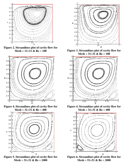
The fluid flow in a square cavity is the best problem to verify numerical results [4-7, 11]. Therefore flow field in a cavity was simulated. The velocity field at the top moving wall of the cavity shows a large recirculation region inside the cavity. With increasing moving wall velocity and the Reynolds number value, additional smaller recirculation zones appear in the corners of the cavity.

(19)

Figure 2. Streamlines plot of cavity flow for

Mesh = 11×11 & Re = 100 Figure 3. Streamlines plot of cavity flow for Mesh = 31×31 & Re = 100

Figure 4. Streamlines plot of cavity flow for Mesh = 31×31 & Re = 400

(20)

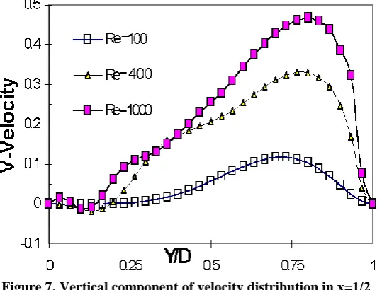
direction on the top is equal to the input value and at the solid boundary is zero. The vertical component is trivial compared with horizontal one due to swirling nature of flow. In other words the velocity fluctuations in the vertical direction are significantly higher than those in the horizontal direction.

Figure 7. Vertical component of velocity distribution in x=1/2

Figure 8 shows velocity field distribution at the centre of the cavity in x direction at y=D/2 (with D as the height of the cavity). On the solid boundary, the values of the velocity components are zero and the results show the nature and behavior of the flow very well.

Figure 8. Horizontal component of velocity distribution in y=D/2

(21)

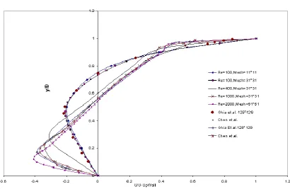
Figure 9. Comparison of vertical component of velocity distribution in x=L/2 with Ghia & Chen results

4. Conclusion

We have extended a vorticity-Stream function formulation for computation of unsteady incompressible fluid flow based on an alternating direction implicit. Therefore in this research, analysis of flow field in a cavity with different values of the Reynolds numbers 100, 400, 1000 and 2000 was carried out by solving the NSE using and Vorticity–Stream function formulation and the ADI algorithm. The solutions for wall cavity flow are stable and convergent. Moreover, we believe that more work need to be done in this subject. Therefore, we will try to solve this problem by using an ADI finite difference method. To this, special formulations with different degrees of approximation which satisfy the boundary conditions are obtained. Finally, comparing the results with the benchmarks show that alternating direction implicit is an effective and suitable formulation for the solution of NSE. Therefore the method is an efficient with promising results.

5. References

1. Ghia U, Ghia K N, Shin C T. (1982). High-Re solution for incompressible flow using the Navier-Stokes equations and a multigrid method. Journal of Computational Physics, 48(3), 387-411.

2. Chen KH, Pletcher RH, (1991), Primitive variable strongly implicit calculation procedure for viscous flows at all speeds. AIAA Journal, 29(8), 1241-1249.

3. Driesen C H, Kuerten J G M, Streng M. (1998). Low-Reynolds-number flow over partially covered cavities. Journal of Engineering Mathematics, 34(1-2), 3–21.

4. Koseff J R, Street R L. (1984). On end wall effects in a lid-driven cavity flow. Journal of Fluids Engineering, 106(4), 385–389.

(22)

quantitative observations. Journal of Fluids Engineering, 106(4), 390–398.

6. Prasad A K, Koseff J R. (1989). Reynolds number and end-wall effects on a lid-driven cavity flow. Physics of Fluids, 1(2), 208–218.

7. Aidun C K, Triantafillopoulos N G, Benson J D. (1991). Global stability of a lid-driven cavity with through flow: flow visualization studies. Physics of Fluids, 3(9), 2081–2091.

8. Gürcan F. (2003). Effect of the Reynolds number on streamline bifurcations in a double-lid-driven cavity with free surfaces. Computer & Fluids, 32(9), 1283–1298.

9. Erturk E, Gokcol O. (2007). Fine grid numerical solutions of triangular cavity flow. The European Physical Journal Applied Physics, 38(1), 97–105.

10. Agarwal R K. (1981). A third-order-accurate upwind scheme for Navier-Stokes solutions at high Reynolds numbers. AIAA Paper No. 81-0112, 15 p.

(23)

Wave Evolution in Water Bodies using Turbulent MPS

Simulation

Hanifeh Imanian1 Morteza Kolahdoozan2 Amir Reza Zarrati3

Abstract

Moving Particle Semi-implicit (MPS) which is a meshless and full Lagrangian method is employed to simulate nonlinear hydrodynamic behavior in a wide variety of engineering application including free surface water waves. In the present study, a numerical particle-based model is developed by the authors using MPS method to simulate different wave problems in the coastal waters. In this model fluid and solid are treated as separate phases and governing equations of momentum and continuity are solved for them concurrently. For simulations of turbulent wavy flows, constant eddy viscosity, Prandtl’s mixing length theory and k-ε models were considered. In addition, higher order of MPS operators was applied to suppress numerical oscillation in comparison with previous studies. The developed method was applied to some cases, including still water reservoir, solitary wave propagation in a tank, tsunami run-up on an inclined wall and wave generation due to the landslide. Evaluation of the developed model results, in compare with data cited in the literature showed enhancement in the accuracy of the developed numerical model especially in compare with existing inviscid models. Besides, the numerical tests results have shown that applying k-ε turbulence model, have equipped MPS model with a useful, powerful and reliable tool for simulating water free surface in wave motion, wave impact and the breaking process.

Keywords: numerical modeling, Lagrangian approach, Moving Particle Semi-implicit (MPS) method, turbulence modeling, wave evolution

Received: 18 March 2018; Accepted: 25 May 2018

1_{Assistant professor, Department of Civil Engineering, Engineering Faculty, Alzahra University, Tehran,}

Iran, [email protected] (Corresponding author)

2_{Associate professor, Department of Civil and Environmental Engineering, Amirkabir University of}

Technology, Tehran, Iran, [email protected]

3_{Professor, Department of Civil and Environmental Engineering, Amirkabir University of Technology,}

(24)

1. Introduction

Owing to commercial and economical role in coastal areas, studying waves have significant hydraulic importance especially in marine environments and estuaries. Hydrodynamic simulation of wave mechanics is however difficult due to complexity of their boundary conditions which are incorporated with an arbitrary moving surface. Despite the great advances in numerical modeling, it is still difficult to simulate free surfaces or solid- fluid interactions like wave impact to coastal structures.

Recently, Lagrangian approaches are applied in free surface modeling [1]. According to this approach, the study area is divided into a number of particles and the governing equations of flow are discretized and solved for each particle [2]. In particle-based methods no mesh generation is required and therefore free surface can be predicted by tracking fluid particle positions in each time step. This means no additional equation is necessary to be solved for free surface prediction. Since no mesh is necessary, the numerical dispersion errors, which are related to mesh generation, are eliminated.

The ﬁrst ideas in this way were proposed by Monaghan in the area of astrophysical hydrodynamic problems with the method called Smooth Particle Hydrodynamics (SPH) [2]. This method was later generalized to ﬂuid mechanic problems. One of the latest particle based methods is Moving Particle Semi-implicit (MPS) which was originally introduced by Koshizuka and Oka [3].

MPS method is applied for modeling a number of hydraulic phenomena such as dam break (Koshizuka et al.), breaking waves (Koshizuka et al.; Gotoh and Sakai and Gotoh et al.), jet breakup (Shibata et al.) and flow over spillways (Shakibaeinia and Jin) [4, 5]. Moreover, Gotoh et al. and Gotoh and Sakai developed a multi- phase MPS model for simulating gas- liquid and solid- liquid problems, sediment transport and floating bodies [1]. Ataie-Ashtiani and Farhadi compared different kernel functions and introduced a formulation for increasing the stability of the MPS model [6]. Zhang et al. proposed a new Laplacian model and used MPS method in simulating heat transfer problems [7]. Shibata and Koshizuka applied a 3D model to simulate behavior of rushing water into the ships and predicted the impact pressure on the deck [8]. Fayyaz added several variables such as surface tension to the multi- phase MPS model to improve its stability and accuracy [9]. Kondo et al. introducing an artificial pressure, suppressed pressure oscillation which is usually observed in MPS modeling [10].

Khayyer and Gotoh worked on conservation of momentum and introduced new formula for calculating pressure gradient and allowed a slight compressibility to suppress its fluctuations [5]. Later on, Khayyer and Gotoh proposed a higher order Laplacian formulation for stabilization and enhancement of pressure calculation [11]. Shakibaeinia and Jin replaced incompressibility in the original MPS model with a weakly incompressible model, by particle recycling strategy for boundary condition [12]. Tanaka and Masunaga tried to obtain a smooth pressure variation both in time and space and eliminate its oscillation [13]. Slamming problems such as liquid- liquid and solid- liquid collision were simulated by Lee et al. using MPS method [14]. To suppress the unphysical pressure oscillation, Kondo and Koshizuka proposed a new formulation for the source term of Poisson equation of pressure [15].

(25)

eddy viscosity assumption to simulate wave breaking on the beach by SPH method [17]. Two-equation k-ε turbulence model was chosen by Shao to couple with SPH scheme for simulating wave breaking on a slope [18]. To investigate the properties of the plunging waves, Shao and Ji combined numerical method of SPH with LES and used Smagorinsky model to simulate turbulence stresses [19]. Violeau and Issa reviewed turbulent models adapted to the SPH method from simplest model of mixing length to more sophisticated ones such as EARMS or LES [20].

In contrast with SPH, MPS method is usually used for modeling inviscid free surface flows and attempts to apply turbulence effects in these models has been very limited [21, 22, 23]. In the governing equations of Large Eddy Simulation, only Reynolds stress is a new term. So compared with the RANS, the governing equations of LES is easier to handle in MPS method. Gotoh et al. 2001 demonstrate advantage of simulation of free surface flow by LES simulation in MPS [24]. Fayyaz and Kolahdoozan tried to add the viscous effects of flow by means of constant eddy viscosity to their phase MPS model [25]. Shirazpoor developed their multi-phase MPS method using Prandtl’s mixing length theory and k-ε model in dam break problem [26, 27]. Pan et al. introduced an area-time average method to reduce the pressure fluctuation in MPS in their MPS-LES model and applied it to a 2D sloshing simulation [28]. Mosaffa and Tang et al. defined a refinement algorithm based on the particle splitting and increased the resolution of the whole simulation region in MPS multi-resolution model [29, 30]. Ikari et al. developed an erosion sub-model in their MPS model for analysis of large deformations of soil, due to wave induced erosion in sea cliffs. The model was further enhanced by utilizing sub-particle-scale suspended sediment load sub-model together with advection-diffusion equation by [31]. Harada et al. developed a DEM-MPS coupled method for reproduction of swash beach sediment transport processes in a gravel beach and investigated the formation/deformation processes of step series on the riverbeds in mountain [32, 33]. Gotoh and Khayyer provided an up-to-date comprehensive review on latest advancements related to particle methods with applications in coastal and ocean engineering [34]. They also highlighted future perspectives for further enhancement of applicability and reliability of particle methods for coastal and ocean engineering.

In this study, a particle-based numerical model is presented using MPS method to simulate different wave problems. The authors have developed their own code to simulate viscous fluid flow in the coastal waters. They have applied governing equations on fluid particles rather than mesh and solved them by MPS method to predict hydrodynamic parameters of solution domain. The effect of turbulence is calculated using three turbulence closures including constant eddy viscosity; Prandtl’s mixing length and k-. Herein, results obtained for a number of wave problems from different turbulence closures combined with the developed MPS model are compared with experimental data or analytical solutions cited in the literature. It was found that considering turbulence effects improves the stability, accuracy and capability of the MPS model.

2. Governing Equations

Governing equations of viscous fluid flow include continuity and momentum equations can be represented as follows:

1_{⁄ D}_ρ ρ Dt

⁄ + ∇𝐮 = 0 (1) D𝐮

Dt

⁄ = − 1⁄ ∇p +_ρ ν_t∇2_{𝐮 + g (2)} where u= velocity vector, t= time, ρ= fluid density, P= pressure, 𝜈𝑡= fluid eddy-viscosity and g= gravitational acceleration.

(26)

which contains both the static and dynamic parts. Thus, by solving Poisson equation, the pressure term can be calculated for all particles. Poisson equation rewrites as follows [3]:

∇2_{P = ∆}ρ ∆t2

⁄ (3) In the MPS method, free surface is predicted automatically when all particles position were specified.

2.1. Model Discretization

In the MPS method the equations of continuity and momentum are converted to interaction equations of particles using different operators. All interactions between particles are limited to a specific distance known as efficient radius. The weighting of different neighboring particles within the efficient radius on the desired particle is calculated based on Kernel functions. In the present study following basic interaction model is used as the Kernel function [5]:

w (r) = {

re_{⁄ − 1 0 < r r}_r e ⁄ ≤ 1 0 1 < r r⁄e

(4)

where r= distance between two particles i and j, 𝑟𝑒= efficient radius and w= Kernel function. This function is effective for saving computational time and memory and is efficient for avoiding clustering of particles and improves numerical stability [17].

The particle number density, actually a weighted average, can be deﬁned in the following form by using the kernel function [3]:

〈n〉i= ∑ w(|rj≠i j− ri|) (5) where 𝑛_𝑖 is the density of particle i in location 𝑟_𝑖.

Since the fluid density is proportional to the particle number density [3], the continuity equation is satisfied if the particle number density is constant in incompressible fluids [6]. This constant value is denoted by 𝑛0_{and is called standard density. For 𝑛}0_{we use particle number} density in the initial state.

A gradient vector is evaluated between two neighboring particles. The gradient operator is modeled using the weight function and conserve linear and angular momentum. It can be expressed as [5]:

〈∇ϕ〉_i_{= d n}⁄ ∑ [₀ (ϕi+ ϕj) − 2ϕ̂i

|r_j− r_i|2

⁄ (r_j− r_i)w(|r_j− r_i|)]

j≠i (6)

where 𝜙= a physical quantity, 𝑑= number of dimension (for two dimensions is replaced with 2), 𝑟_𝑖= location vector for particle i, and 𝜙′= minimum amount of 𝜙 belonging to the neighboring particles in the efficient radius:

ϕ_i′ _{= min(ϕ}

j) for {w(|rj− ri|) ≠ 0} (7) The presented Laplacian model has a conservative form and can be written as [3]:

〈∇2_ϕ〉

i= 2d n⁄ 0_λ∑ [(ϕj≠i j− ϕi)w(|rj− ri|)] (8) In the above equations, λ is a coefficient defined as:

λ= ∫ w(r)r2dv

∫ w(r)dv

⁄ (9)

2.2. Turbulence Closures

Since the flow in this study is viscous and turbulent, Prandtl’s mixing length theory and k-

(27)

domain.

According to Prandtl’s mixing length model [35,36] which is widely used in estuaries and coastal waters [37] eddy viscosity νt can be written as:

ν_t,i=κu_∗iz_i(1 − zi H

⁄ ) (10) where, 𝜈𝑡,𝑖= turbulent eddy viscosity for particle i, = von Karman’s constant, 𝑢_∗𝑖= shear velocity for particle i, 𝑧_𝑖= vertical distance of particle i from the bed and H= total water depth.

According to k- turbulent model [38] eddy viscosity 𝜈𝑡 can be written as: ν_t,i= C_μki2

εi

⁄ ₍₁₁₎

where 𝑘_𝑖= turbulence kinetic energy for particle i, 𝜀_𝑖= energy dissipation rate for particle i and 𝐶𝜇 is a constant= 0.09.

Lagrangian form of convection equation for turbulence kinetic energy, k can be written as [20, 38]:

Dk Dt

⁄ = Pk−ε+ ∇[(ν+νt⁄ )∇k] (12) σ_k where 𝜎_𝑘 is a constant =1.0.

This equation is analogous to the convection-diffusion equation where the production rate of kinetic energy 𝑃_𝑘 is similar to the source term, while energy dissipation  is similar to the sink term P. In the MPS method the convection equation for k reads as:

Δk Δt

⁄ = P_ki−ε_i+2dνk,i n0_λ

⁄ ∑ [(kj≠i j− ki)w(|rj− ri|)] (13)

where:

νk,i =ν+νt,i⁄σ_k (14) in vector form, the source term P is [20]:

𝑃 =ν_tS2₍₁₅₎ However, for preventing any overestimation of k in cases with high rates of strain, the non-isotropic turbulence should be limited. Therefore, a linear strain variation rate is considered for high deformations and the source term of particle i is limited as follows [20]:

P_ki= min (√Cμ, CμSiki⁄ ) kε_i iSi (16) For calculating the scalar mean rate of strain S one can write [18]:

S = [2(∂u ∂x⁄ )2_{+ 2 (∂v ∂y}⁄ )2_{+ (∂u ∂y}⁄ _{+ ∂v ∂x}⁄ )2]1/2 (17) The energy dissipation rate  can be written as [18, 38]:

Dε Dt

⁄ = ∇[(ν+νt _σ

ε

⁄ )∇ε] +ε⁄ (C_k ε,1Pk− Cε,2ε) (18) where 𝜎𝜀, 𝐶𝜀,1 and 𝐶𝜀,2 are empirical constants= 1.3, 1.44 and 1.92 respectively.

The MPS form of Equation (18) is as follows: Δε

Δt

⁄ =2dνε,i n0_λ

⁄ ∑ [(ε_j≠i _j−ε_i)w(|r_j− r_i|)]+εi k_i

⁄ (Cε,1P_ki− Cε,2εi) (19)

where: ν_ε_,i =ν+νt,i

σε

(28)

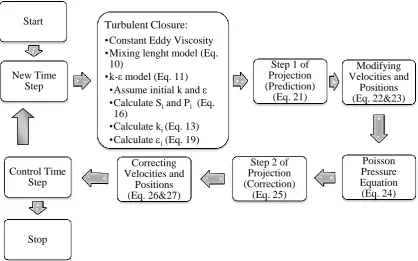
3. Solution Procedure

The governing equations of flow were solved semi-implicitly. To speed up the convergence the Projection method was deployed in which discretization of Navier-Stokes equations were completed in two half time steps. In the first half time step (prediction step) governing equations were solved in the presence of viscosity and gravity terms without enforcing incompressibility, while the pressure were disregarded. In the second half time step (correction step), the results obtained in the previous time step were modified in the presence of pressure gradient. In other words, the pressure term was used to update the particles velocity calculated from the prediction step [15, 17]. In mathematical expression, the Navier-Stokes equations for the first half time step can be written as:

D𝐮 Dt

⁄ =νt∇2𝐮 + g (21) To solve this equation, primarily, eddy viscosity should be computed.

In Prandtl’s mixing length model, the eddy viscosity was computed based on velocity and position of particles according to Equation (10).

In k- model, in each time step, the solution algorithm followed Equation (11) to (20).

After solving Equation (21) explicitly, velocity components variations (u) of all particles were obtained. Then, modified velocity and positions were calculated for each particle as follows:

𝐮t+1/2_{= ∆𝐮}t+1/2_{+ 𝐮}t₍₂₂₎

rt+1/2 _{= 𝐮}t+1/2_{∆t + r}t₍₂₃₎

where 𝒖𝑡, 𝑟𝑡, 𝒖𝑡+1/2, 𝑟𝑡+1/2= current and intermediate particle velocity and position, respectively.

In the prediction step, mass conservation is not satisﬁed. It means the particle number density

𝑛_𝑖𝑡+1/2 that are calculated at the end of ﬁrst half time step deviates from the constant 𝑛0.

Therefore, a second corrective process is required to adjust the particle number densities to initial constant values prior to the time step. In the second half time step, the intermediate particle velocity 𝒖𝑡+1/2_{is updated implicitly through solving the Poisson pressure Equation.}

To calculate particles pressure, Poisson pressure Equation was then solved with the following discretized representation [11]:

〈∇2_P

it+1〉 =ρ⁄_∆t2ni

t+1/2_{− n}0

n0

⁄ ₍₂₄₎

where ∆𝑡= calculation time step and t denoted the step of calculation.

Since explicit calculation of Poisson pressure equation leads to model instability, it is recommended to solve it in full implicit form as a linear equations system. One of solving methods for this linear system is Cholesky solution [39].

Finally, given the amount of particles velocity components and position at time t+1/2 and pressure value, the second time step of Projection method was enforced. In this stage, pressure was included in the momentum equations in the following form:

ρD𝐮⁄_Dt= −∇p (25) This equation was solved implicitly and new velocity components and particle positions in the next time step were calculated as follows:

(29)

Figure 1. Solution algorithm of the present MPS model

4. Boundary Conditions

4.1. Free Surface

Free surface was defined as the location at which particles density is less than a certain value. Following condition is defined for free surface particle recognition [39]:

n_i< 𝛽n0₍₂₈₎ where 𝛽 = threshold coefficient which is define 0.97 [1, 6, 9].

The standard or zero pressure value would be assigned in each time step to particles in this location and no additional computations were necessary.

4.2. Bed Boundary

Along solid boundary, particles position in the impermeable channel bed and walls were invariable and liquid particles were not able to penetrate into this solid layer. In all time steps, the governing equations were solved for near solid boundary particles to repulse the inner fluid particles accumulating in the vicinity of wall.

To model the no-slip condition in the vicinity of solid boundary, each particle near the boundary was checked for not to penetrate inside the solid boundary [9, 17].

5. Results and Discussion

5.1. Still Water reservoir

A 0.2 m-long reservoir containing still water with 0.2 m depth was modeled by 2601 Start

New Time Step

Turbulent Closure: •Constant Eddy Viscosity •Mixing lenght model (Eq.

10)

•k-ε model (Eq. 11) •Assume initial k and  •Calculate Si and Pi (Eq.

16)

•Calculate ki (Eq. 13)

•Calculate _i (Eq. 19)

Step 1 of Projection (Prediction)

(Eq. 21)

Modifying Velocities and

Positions (Eq. 22&23)

Poisson Pressure Equation

(Eq. 24) Step 2 of

Projection (Correction)

(Eq. 25) Correcting

Velocities and Positions (Eq. 26&27) Control Time

Step

JHS, Vol. 4, Issue 1

Journal of Hydraulic Structures

Department of Civil Engineering

Faculty of Engineering

Shahid Chamran University of Ahvaz

In the name

of GOD

HYDRAULIC

STRUCTURES

CONTENTS

I.

In the name of God

II. Table of Contents

III. Aims and Scope

01

Development of a Direct Explicit Equation

for Hydraulic Design of Semi-elliptical

Channels

08 An Alternating Direction Implicit Method for

Modeling of Fluid Flow

19 Wave Evolution in Water Bodies using

Turbulent MPS Simulation

36 Ocean Currents Modeling along the Iranian

Coastline of the Oman Sea and the

Northern Indian Ocean

55 Study of Streamlines under the Influence of

Displacement of Submerged Vanes in

Channel Width, and at the Upstream Area of

a Cylindrical Bridge Pier in a 180 Degree

Sharp Bend

75 Frequency domain analysis of transient flow

in pipelines; application of the genetic

programming to reduce the linearization

errors

Aims and Scope

General Information

Development of a Direct Explicit Equation for Hydraulic

Design of Semi-elliptical Channels

Abstract

1. Introduction

2. Design Method

1

AS

R

n

Q



n

S

3. Calculation of Flow Cross Sectional Area and Wetted-Perimeter

)

(

)

(

)

(

)

(

x

y

x

x

y

y

L



















(

x

,

y

)

(

_