Numerical Simulation of Flow Pattern around the Bridge Pier with Submerged Vanes

(1)

AUTUMN 2016, Vol II, No II, JOURNAL OF HYDRAULIC STRUCTURES Shahid Chamran University of Ahvaz

Journal of Hydraulic Structures J. Hydraul. Struct., 2016; 2(2):46-61

DOI: 10.22055/jhs.2016.12856

Numerical Simulation of Flow Pattern around the Bridge Pier

with Submerged Vanes

Sajedeh Haji Azizi1 Davood Farsadizadeh2 Hadi Arvanaghi3 Akram Abbaspour4

Abstract

Bridges are very important for establishing communication paths. For this reason, it is important to control scour around bridge piers. Several methods have been proposed for scour control. One of the most useful methods is the use of submerged vanes. In the other hand, laboratory circumstances force many considered effective factors to be skipped in the scour phenomenon. In this situation, the importance of using numerical models would appear even more. In this research, numerical simulation of the flow pattern around the piers surrounded by submerged vanes has been carried out. For this purpose, the structure simulated in three dimensions using Fluent software. K-ε turbulence model with VOF and mixture models for multiphase flow simulation were applied. Afterward analysis of the water surface profiles, velocity distribution profiles, and shear tension of the bed in multiple placements conditions including multiple vanes within two flow intensity and two different angles were performed. The results showed that there is a good agreement between numerical and experimental results. The best models in this research were found to be Realizable k-ε turbulence model with VOF multiphase model for water surface profile and velocity distribution profiles. The maximum extracted relative errors for water surface profiles and velocity distribution profiles were 2.23% and 2.92%, respectively. Also, analysis of the counts and placement angles showed that 6 vanes rather to 2 and 4 vanes and also angle of 30 degrees rather to angle of 20 degree performs better in action. The other results of this study, are no change in water surface profiles, reduction of the velocity and the amount of shear stress around the piers in different placement conditions including multiple submerged vanes.

Keywords: Scouring, Flow pattern, Bridge pier, Numerical simulation, Submerged vanes Received: 06 September 2016; Accepted: 15 November 2016

1_{Department of Water Engineering, University of Tabriz, Tabriz, 09371676441, [email protected]}

(Corresponding author)

2 _{Associate Professor, Department of Water Engineering, University of Tabriz, Tabriz,}

[email protected]

3_{Assistant Professor, Department of Water Engineering, University of Tabriz, Tabriz, [email protected]} 4 _{Assistant Professor, Department of Water Engineering, University of Tabriz, Tabriz,}

(2)

1. Introduction

Bridges are the most important structures of communication which are always subject to degradation. In studies, scour is considered as one of the main reasons of destruction. submerged vanes are used to control the size of the scour hole and to protect the structures. Numerical Study of submerged vanes would be possible by a closer look. Marelius and sinha (1998) experimentally and numerically studied velocity profile around the submerged vanes. Hassanzadeh et al (2006) have developed a numerical model to simulate the flow pattern around bridge piers. Ariyanfar and Shafai Bajestan (2008) numerically studied the flow pattern around the base of the cylindrical piers using Fluent model. Besharati Givi and Hakim Zadeh (2009) simulated cylindrical pier in models three dimensions using Fluent software. Alamatiyan and Jafarzadeh (2009) they studied the numerical model of flow conditions around the bridge piers. Sarveram et al (2008) studied the numerical simulation and flow velocity distribution around bridge pier. Kariminia and Salehi Neyshabouri (2011) simulated the backwater phenomenon for bridge pier using Fluent software. Asadi Partov et al (2012) studied numerical simulation of flow pattern in a direct channel and the effect of bridge pier diameter on it. Kalali et al (2012) studied the numerical simulation of the flow pattern around slant bridge piers. Hoshmand et al (2013) studied three-dimensional numerical modeling of the flow around the bridge pier in meandering beds. Yen et al (2001) simulated bed change and flow pattern in the cylindrical bridge pier using Flow-3D software and a combination of three-dimensional flow model and scour model. Roulund et al (2002) simulated flow around bridge pier by three-dimensional numerical model. In the present study, the flow pattern around bridge piers including submerged vanes simulated and assessed. This study was carried out with a CFD program, which uses the finite volume method to solve 3D Reynolds averaged Navier Stokes (RANS) equations for this model. The free surface levels computed using VOF (volume-of-fluid) method and compared with experimental data.

2. Materials and Methods

2.1. Experimental Procedure

The experiments carried out by Shojaei (2009) in a metal glass flume with a rectangular cross-section. The flume was 0.8 m wide, 0.5 m deep and 8 m long. The slope of the channel was 0.001. A cylindrical steel pipe with diameter of 0.06 m used to model the pier. Submerged vanes models made in rectangular square form. The submerged vanes was 0.001 m wide, 0.03 m deep and 0.09 m long. The discharge was measured by a rectangular weir placed at the end of channel. Fig. 1 shows the submerged vanes and the pier parameters. In all experiments, according to the calculations u∗⁄u∗c= 0.9, flow depth equaled to 0.147 m and discharge is considered 0.03 m3⁄sec. Also, with depth of 0.147 m has been considered which is the required condition in order to avoid flow depth affecting on scour hole depth. In all experiments, the flow was turbulent. The recognition criterion in this type of flows is Reynolds number, which is defined as Re =

(3)

Table 1. The variable parameters in experiments submerged vanes in front of the base

Geometric variables

n 2, 4 ,6

α 20°, 30°

hydraulic

variables 𝑉 𝑉⁄ 𝑐 0.8 , 0.95

Fig. 1. Plan view of pier and submerged vanes

2.2. Numerical mode

In the present study, the flow pattern around the bridge pier are numerically studied for different flow intensity using the k-ε turbulence models and two-phase flow theory. The numerical solution for most problems are obtained by solving a series of triple differential equations, which is known as the Navier-Stokes equations. These differential equations are about the transition of mass, momentum, and energy.

 

0

     i i u x t  



i j



j i j j i j i j i j

i uu

x x u x u x x p u u x u

t    

                                   _ _ _ _ ) ( ) (

Where 𝑢_𝑖is the average velocity in the direction of i=1, 2 and 3, p is the pressure, μ is the dynamic viscosity of the fluid and 𝑢_𝑖′𝑢_𝑗′ is Reynolds stress term. So, this system of equations is not definite and Reynold’s stress should be calculated using proper turbulence model.

2.2.1. Volume of Fluid (VOF)

In computational fluid dynamics, the volume of fluid (VOF) method is a free-surface modelling technique for tracking and locating the free surface levels. Determining the free surface levels by VOF method requires a function F which is known as Volume of Fraction (VOF). The differential function in two-dimensional mode presented as following:

𝜕𝐹 𝜕𝑡 + 𝑢

𝜕𝐹 𝜕𝑥+ 𝑣

𝜕𝐹 𝜕𝑦= 0

(4)

Reconstruction scheme.

Fig. 2. (a) Actual interface shape (b) interface shape represented by the Geometric reconstruction scheme (c) interface shape represented by the donor-acceptor scheme (Fluent, 2006)

2.2.2. Realizable k-ε Model

The realizable k-ɛ model contains a new formulation for the turbulent viscosity and a new transport equation for the dissipation rate, ɛ, that is derived from an exact equation for the transport of the mean-square vorticity fluctuation. The transport equations of Realizable k-ε model are as following:

𝜕

𝜕𝑡(𝜌𝑘) + 𝜕

𝜕𝑥𝑗(𝜌𝑘𝑢𝑗) =

𝜕 𝜕𝑥𝑗[(𝜇 +

𝜇𝑡

𝜎𝑘)

𝜕𝑘

𝜕𝑥𝑗] + 𝑃𝑘+ 𝑃𝑏− 𝜌𝜀 − 𝑌𝑀+ 𝑆𝑘

𝜕 𝜕𝑡(𝜌𝜀) +

𝜕

𝜕𝑥𝑗(𝜌𝜀𝑢𝑗) =

𝜕 𝜕𝑥𝑗[(𝜇 +

𝜇𝑡

𝜎𝜀)

𝜕𝜀

𝜕𝑥𝑗] + 𝜌𝐶1𝑆𝜀+ 𝜌𝐶2

𝜀2

𝑘 + √𝜐𝜀+ 𝐶1𝜀 𝜀

𝑘𝐶3𝜀𝑃𝑏+ 𝑆𝜀

Where, 𝐶₁= max [0.43 ∙ 𝜂

𝜂+5] 𝜂 = 𝑆 𝑘

𝜀 𝑆 = √2𝑆𝑖𝑗𝑆𝑖𝑗 𝐶1𝜀 = 1.44 𝐶2= 1.9 𝜎𝑘= 1.0 𝜎𝜀 = 1.2

In these equations, 𝑃𝑘 represents the generation of turbulence kinetic energy due to the mean velocity gradients, calculated in same manner as standard k- ε model. 𝑃_𝑏 is the generation of turbulence kinetic energy due to buoyancy, calculated in same way as standard k- ε model.

The differential equation for turbulence viscosity,𝜇_𝑡 ,are as following: 𝜇_𝑡 = 𝜌𝐶_𝜇𝑘

2

𝜀

Where, 𝐶_𝜇 = 1

𝐴0+𝐴𝑠𝑘𝑢∗_𝜀

𝑈∗_{= √𝑆}

𝑖𝑗𝑆𝑖𝑗+Ω̃ Ω𝑖𝑗̃𝑖𝑗 Ω̃ = Ω𝑖𝑗 𝑖𝑗− 2𝜀𝑖𝑗𝑘𝜔𝑘 Ω𝑖𝑗 = Ω̅̅̅̅ − 𝜀𝑖𝑗 𝑖𝑗𝑘𝜔𝑘

Where Ω̅̅̅̅_𝑖𝑗 is the mean rate-of-rotation tensor viewed in a rotating reference frame with the angular velocity 𝜔𝑘. The model constants 𝐴0 and 𝐴𝑠 are given by: 𝐴0= 4.04 𝐴𝑠= √6 𝑐𝑜𝑠𝜙

𝜙 =1₃𝑐𝑜𝑠−1_(√6𝑊)_{𝑊 =}𝑆𝑖𝑗𝑆𝑗𝑘𝑆𝑘𝑖

𝑆̃3 𝑆̃ = √𝑆𝑖𝑗𝑆𝑖𝑗 𝑆𝑖𝑗=

1 2(

𝜕𝑢_𝑗 𝜕𝑥𝑖+

𝜕𝑢_𝑖 𝜕𝑥𝑗)

2.2.3. Model geometry and boundary conditions

(5)

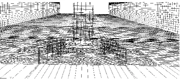
thickness of the vanes (1 mm) the tetrahedron (triangular) elements was used. In order to make acceptable mesh in the pier area the Quad-Pave algorithms and in other parts the Quad-Map algorithm was used. Meshing volumes in the pier area with algorithms Hex-Cooper and in other parts of the Hex-Map algorithm was performed. In the final step, the boundary conditions for walls, pier and submerged vanes, input and output page and also velocity inlet defined and saved by *.msh format in order to import it to Fluent software. One of the constructed mesh files in Gambit presented as Fig. 3.

Fig. 3. Grid for pier area and four submerged vanes

3. Results and Discussions

3.1. Calibration of the numerical model

In order to calibrate a numerical model, the experimental results of Arvanaqhi (2009) is used. His experiments in rectangular channel with a length of 10 meters, width of 0.25 m and a height of 0.50 m was peformed. Diameter of the model pier used in this series of experiments was 0.012 m. In order to calibrate the numerical model, depth and velocity parameters (profiles of water level and flow velocity profiles), experimental and numerical models compared. In experimental models, the water depth measured by bathymetry sensors at the top of the channel and upstream of the bridge pier, and it was controlled and corrected using gauge surface. as well as, the horizontal component of the flow velocity (Vx) around bridge pier, extracted by Micro Propeller in two model V/Vc within accuracy of 1.0 centimeters per second. In order to calibrate, the velocity distribution profile, along the longitudinal axis of channel (Z = 0) and in two sections by distance 3 and 10 cm from the center of the bridge piers in the upstream and in V / Vc = 0.95 was investigated. Also, the water surface profile on two axes Z = 0 (central axis) and Z = ± 3 cm (lateral axis) was extracted and compared to experimental results.

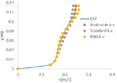
Initially to choose the best model of turbulence, k-ε turbulence model using three models of Standard, RNG and Realizable investigated and the results of numerical models compared to experimental results and Relative Average Error (RAE) was calculated. In the following equation (𝑣𝑝) and (𝑣𝑛) respectively, are flow velocity in the physical models and the Numerical models.

(𝑅𝐴𝐸)𝑉% =

∑𝑁𝑖=1|(𝑣𝑝𝑖− 𝑣𝑛𝑖)|

∑𝑁𝑖=1𝑣𝑝𝑖

× 100

(6)

amount of error in the model it can be used to determine the Reynolds stress and viscosity of vortices more accurately, and as a result solving the momentum equation more accurately.

Fig. 4. Comparison of the velocity profile with a variety of k-ε turbulence models and experimental results

Table 2. The error rate (RAE %) of k-ε turbulence models

Realizable k-ε Standard

k-ε RNG

k-ε turbulence

models

1.674 3.476

2.81 5 Error (%)

After selecting the best model of turbulence, comparison of the horizontal velocity (Vx) was conducted in two cross-sections (figures 5 and 6). The results show that the numerical models are in good agreement with physical model, So that the numerical models error in two sections by distances of 3 and 10 cm from the center bridge pier, respectively, 2.29 % and 1.76 % were calculated which is relatively neglectable error. The bigger value for error in section 3 cm, indicate more turbulence at this point.

Fig.5. Comparison of the Vx in a distance of 3 cm

from the pier

Fig.6. Comparison of the Vx in a distance of 10 cm

from the pier

In this section, to increase the accuracy and reduce computational process, assessment of the

y = 1.0182x R² = 0.9879

0 0.05 0.1 0.15 0.2 0.25 0.3

0 0.1 0.2 0.3

n

u

m

erical

experimental

y = 1.0027x R² = 0.9929

0 0.05 0.1 0.15 0.2 0.25 0.3

0 0.1 0.2 0.3

n

u

m

erical

(7)

mesh size effect was issued. For this purpose, modeling the water level changes by using different mesh size has been done and the results were compared with experimental results of Arvanaghi (2009). Numerical analysis results show (Table 3) that with decrement of the mesh size to a specified size (increase the counts of meshes), their results would change and get closer to the true value, but further that, there isn’t significant change in the results and only increase the model runtime. So, the mesh count of 81000 selected. To verify the authenticity of meshes, the relative average error (RAE) and standard root mean square error (RMSE) was used. In the following formula (yp) and (yn), respectively, is water depth in physical model and water depth in numerical model. The equation is as follows:

(𝑅𝐴𝐸)𝑦% =

∑𝑁_𝑖=1|(𝑦_𝑝𝑖− 𝑦_𝑛𝑖)|

∑𝑁_𝑖=1𝑦_𝑝𝑖 × 100

(𝑅𝑀𝑆𝐸)𝑦= [ 1

𝑁∑ (𝑦𝑝𝑖− 𝑦𝑛𝑖) 2 𝑁

𝑖=1 ]

0.5

Table 3. errors in simulated water surface profile with different mesh count

RMSE (mm) RAE (%)

Counts of mesh

9.18 6.12

37000

6.51 4.07

52000

1.67 1.05

81000

2.71 1.43

100000

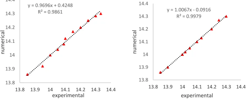
After selecting the best counts of meshes, simulation and analysis of water surface profile in the central axis and two lateral axes around the bridge pier was done. The results showed that the water surface profiles are in good agreement with physical models (Figure 7 and 8) and the error, were calculated in the two axes 0 and ±3 cm from the center pier respectively, 2.23% and 2.09%, whereas considering the fact that some calculation of water surface profiles, done through interpolation due to mixture interface of water and air, but errors were neglectable.

According to the results above, it can be said that the Fluent software has the ability to simulate the flow pattern and the results can be trusted due to the high relative accuracy.

Fig 7. Comparison of the flow depth in lateral axis Fig 8. Comparison of the flow depth in central axis

3.2. Water Surface Profile

The free surface profiles obtained by the Volume of Fluid (VOF) method which presented in Figs. 9 and 10. In the central axis of the channel (Figs. 9), when the water flow approaches to the

y = 0.9696x + 0.4248 R² = 0.9861

13.8 13.9 14 14.1 14.2 14.3 14.4

n

u

m

erical

experimental

y = 1.0067x - 0.0916 R² = 0.9979

13.8 13.9 14 14.1 14.2 14.3 14.4

n

u

m

erical

(8)

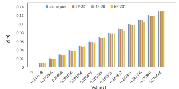
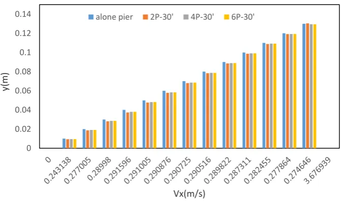
bridge pier, due to decrement of the flow velocity, water depth increase in front of the pier. Also On the back of pier due to constriction section, the flow velocity increases and water level decrease. In the lateral axis (Z = + D) increasing and decreasing water levels in the upstream and downstream pier does not happen. The reason of that is the long distance between the axis and bridge pier (Fig 10). The results showed that the counts of submerged vanes as well as their angle, has no effect on the water surface profiles, so it can be said that submerged vanes like collar have no effect on the water level (in accordance with the results Arvanaqhi, 2009).

Fig.9. comparison of the water surface profile at Z = 0, 𝑉/𝑉𝑐 = 0.95 , 𝛼 = 30˚

Fig.10. comparison of the water surface profile at 𝑍 = +𝐷, 𝑉/𝑉𝑐 = 0.95 , 𝛼 = 30˚

3.3. Flow Velocity Distribution

In this section, it has been dealt with the velocity distribution with the Realizable k-ε turbulence model and 𝑉 𝑉⁄ = 0.95_𝑐 in different sections which indicated in Figure 11. In order for better understanding, changes in velocity, the results from added vanes as an obstacle in the flow direction, initially dealt with the horizontal velocity component distribution of single bridge pier (without submerged vanes) and afterwards channel modeling has been done with bridge pier and submerged vanes.

0 0.04 0.08 0.12 0.16 0.2

0 0.2 0.4 0.6 0.8 1 1.2 1.4 1.6 1.8 2

y(m

)

x(m)

without submerged vanes 2 submerged vanes

4 submerged vanes

6 submerged vanes

0 0.04 0.08 0.12 0.16 0.2

0 0.2 0.4 0.6 0.8 1 1.2 1.4 1.6 1.8 2

y(m

)

x(m)

without

submerged vanes

2 submerged vanes

4 submerged vanes

(9)

Figure 11. Axes of velocity Distribution

3.3.1. The horizontal Velocity Component Distribution

In this section, initially the impact of existence or absence of the submerged vanes on the velocity profile at the central axis (𝑍 = 0) and lateral axis on the right (𝑍 = +𝐷) examination has been performed. Then comparison of the angle impact of the submerged vanes (20 and 30 degrees) and also their counts (2, 4 and 6), on the distribution of the horizontal velocity component in the introduced axis, is taken into consideration. According to Table 4, Figures 12, and 13, the horizontal velocity component at the pier with submerged vanes is less than the pier without submerged vanes, Therefore, as a conclusion installation of submerged vanes around the bridge pier, would reduce the velocity in channel axis’s, which would result in reducing local scour around bridge piers.

Table 4. The mean values of velocity (m / s) in two axes 𝑍 = 0 and 𝑍 = +𝐷

(

𝑚 𝑠

) The mean values of velocity Location of the

vanes _{𝑍 = +𝐷} _{𝑍 = 0}

0.19203 0.2899

alone pier

0.1411 0.2621

2P-30˚

0.1301 0.2141

4P-30˚

0.1174 0.1282

6P-30˚

0.1485 0.2637

2P-20˚

0.1391 0.2231

4P-20˚

0.1320 0.1405

6P-20˚

(10)

Fig 13. Comparison of the horizontal velocity component in 𝛼 = 20˚ , 𝑍 = +𝐷

Checking the angle impact of the submerged vanes, in the axis’s of 𝑍 = 0 , +𝐷 indicates that the horizontal velocity component distribution at the angle of 30˚ decreases rather to 20˚, Therefore, it can be concluded that an angle of 30˚ is better and more effective than angle of 20˚ in the velocity decrement in undermining local scour around bridge piers (Table 5). Reason for irregularity of the velocity distributions could be linked to the angles and the counts of submerged vanes. (Fig 14).

Table 5. The mean values of velocity (m / s) in order to comparison the angles of submerged vanes on two axes Z = 0 , +D

(

𝑚 𝑠

) The mean values of velocity Location of the vanes

𝑍 = 0 𝑍 = +𝐷

0.1687 0.2635

single pier

0.1468 0.2626

2P-30˚

0.1304 0.2135

4P-30˚

0.1286 0.1628

6P-30˚

0.1532 0.2775

2P-20˚

0.1373 0.2184

4P-20˚

0.1301 0.1989

6P-20˚

Fig 14. Comparison of the angle of submerged vanes in 𝛼 = 20˚ , 𝑍 = +𝐷

0 0.02 0.04 0.06 0.08 0.1 0.12 0.14

0 0.1 0.2 0.3 0.4

y(m

)

Vx(m/s)

6P-30'

(11)

Also, checking the impact of the submerged vanes counts on the axis’s 𝑍 = 0 , +𝐷 resulted in the fact that six vanes have greater impact on reducing the horizontal velocity component around

the pier and lead to better scour control (Figures 15 and 16)

Fig 15. Comparison of the horizontal velocity component in 𝛼 = 30˚ , 𝑍 = 0

Fig 16. Comparison of the horizontal velocity component in 𝛼 = 30˚ , 𝑍 = +𝐷

It is worth noting that the effect of lower vanes in the axis 𝑍 = 0, more near to the bed observed with better performance in reducing scour around the piers. Also, the angle of 30°, has the better performance than the angle of 20° in the horizontal velocity component reducing and consequently reduction of scour.

3.3.2. The Vertical Velocity Component Distribution

In this section, the vertical velocity component distribution at bridge pier, in the two

0 0.02 0.04 0.06 0.08 0.1 0.12 0.14

y(m

)

Vx(m/s)

alone pier 2P-30' 4P-30' 6P-30'

0 0.02 0.04 0.06 0.08 0.1 0.12 0.14

y(m

)

Vx(m/s)

(12)

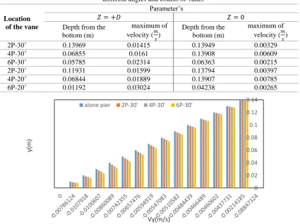
axes 𝑍 = 0 , +𝐷 investigated (Figures 17 and 18). The results showed that installation of submerged vanes reduces the amount of vertical velocity component in the central axis, so that in the case of six vanes with both angel 30 and 20 degree it can be stated that the vertical velocity component of approximately in the depth of 3 cm from the channel bottom (about the height of pages) is equal to zero and indicating that vortexes control is relatively good. Also in the central axis, maximum amounts of velocity, in the case of six submerged vanes, for the two angles 20 and 30 degrees, were respectively 0.00265 m/s and 0.00215 m/s and in the depths of 0.04238 m and 0.06363 m (relative to the channel bottom) occurred, also in this case, the results imply angle of 30-degree for better performance. But in the lateral axis, submerged vanes did not have much success to reduce this component. This result was also in agreement with observations of Shojayi (2009). Because in the series of her experiments, the vanes were only able to control the scour hole at the front of the pier and were not able to control scour at the sides of the pier. Shojayi (2009) used the collar to control the vortices around the pier. Also in Table 6, maximum velocity and depth of all above conditions mentioned, whereas confirms the above results.

Table 6. The maximum values of vertical velocity component and depths of them respectively, at different angles and counts of vanes

Parameter’s

Location of the vane

𝑍 = 0 𝑍 = +𝐷

maximum of velocity (𝑚_𝑠) Depth from the

bottom (m) maximum of

velocity (𝑚_𝑠) Depth from the

bottom (m)

0.00329 0.13949

0.01415 0.13969

2P-30˚

0.00609 0.13908

0.0161 0.06855

4P-30˚

0.00215 0.06363

0.02314 0.05785

6P-30˚

0.00397 0.13794

0.01599 0.11931

2P-20˚

0.00785 0.13907

0.01889 0.06844

4P-20˚

0.00265 0.04238

0.03024 0.01192

6P-20˚

Fig 17. Comparison of the vertical velocity component for 𝛼 = 30˚ , 𝑍 = 0

0 0.02 0.04 0.06 0.08 0.1 0.12 0.14

y(m

)

Vy(m/s)

(13)

Fig 18. Comparison of the vertical velocity component for 𝛼 = 20˚ , 𝑍 = 0

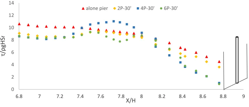
3.4. Shear Stress Distribution

Figures 19 and 20 show Bed shear stress distribution, on the central axis of the channel. In order for better understand, the vertical axis that indicates the amount of stress divided by the total shear stress (𝜏 𝜌𝑔𝐻𝑆⁄ _𝑓) and the horizontal axis that indicates distance to the pier, divided by the channel depth (H) which all are dimensionless. Focusing to the figures 19 and 20 and Table 7 it can be stated in the case of two and six vanes with both of angel 20° and 30°, the maximum shear stress is reduced compare to single pier.

Fig 19. Shear Stress Distribution in 𝛼 = 30˚ , 𝑍 = 0

0 0.02 0.04 0.06 0.08 0.1 0.12 0.14

y(m

)

Vy(m/s)

alone pier 2P-20' 4P-20' 6P-20'

0 2 4 6 8 10 12 14

6.8 7 7.2 7.4 7.6 7.8 8 8.2 8.4 8.6 8.8 9

τ/

ρgH

S

f

X/H

(14)

Fig 20. Comparison of the amounts of shear stress in 𝛼 = 30˚ , 𝑍 = 0

Table 7. The maximum shear stress and its distance from pier in various modes of submerged vanes Shear stress from pier

(𝑵

𝒎𝟐) Distance from pier

(m) maximum shear stress

(𝑵

𝒎𝟐) Location of the vanes

0.068 0.288

0.16 Alone pier

0.0151 0.178

0.142 2P-30˚

0.0153 0.155

0.166 4P-30˚

0.0129 0.189

0.14 6P-30˚

0.0199 0.175

0.135 2P-20˚

0.0215 0.137

0.162 4P-20˚

0.0176 0.178

0.156 6P-20˚

4. Conclusions

Some of the main observations and conclusions can be summarized as follows:

1. Due to the good agreement between numerical and physical models, FLUENT software can be used for determining the parameters that are not measurable in the laboratory for the conditions which measurement accuracy is not enough.

2. It was observed that the fluent software has a high capability to simulate the water surface profiles, so that the error in two axis of 𝑍 = 0 (the central axis) and 𝑍 = ±3 𝑐𝑚 of center bridge pier (lateral axis), were computed respectively, 2.23% and 2.09%. 3. Fluent software was also accurate in simulation of flow velocity profile. So that the error

in the two sections in distance 3 and 10 cm from the center pier and in the central axis channel were calculated respectively, 2.92 % and 1.67 %.

4. By evaluating profiles, the water level in the two central and lateral axis And in two flow intensity were 0.8 and 0.95, the conclusion was that vanes in different flow intensity have little effect on the water surface profile, whereas the maximum created difference observed at 1.564 m from channel beginning part (4 cm from pier) was only 3 mm. 5. Assessing the horizontal velocity component distribution in the channel with and

0 2 4 6 8 10 12 14

τ/ρ

gHSf

x/H

(15)

without the bridge pier and submerged vanes, it was observed that the horizontal velocity component reduced using submerged vanes and it means that the vanes are effective in reduction of velocity and subsequently reduction of local scour around bridge piers.

6. Evaluating and comparing the angle of the submerged vanes on central and lateral axis’s in the channel it was observed that the angle of 30° is better than the angle 20 ° in reduction of horizontal velocity component.

7. Considering the counts of used submerged vanes, it turned out that the counts of 6 was much effective rather than 2 and 4 in reducing of the horizontal velocity component. 8. The studies showed the efficiency of vanes in velocity decrement near to the channel

bed, whereas implies on positive performance of submerged vanes.

9. Assessing the vertical velocity component in the central axis resulted in the fact that in general, existence of vanes reduces this component. So that, placement of six vanes with both angels of 20 and 30 degree in the central axis, the vertical velocity component was approximately equal to zero in 3 cm of the channel bottom (the same height of vanes).

References

1. Fluent 6.3 User’s Guide. (2006). Fluent Incorporated, Lebanon, N.H.

2. Ariyan far, e., and shafaei bajestan, m. (2008). “Numerical Study the flow pattern around the cylindrical bridge piers by fluent”. The Fourth National Congress of Civil Engineering, Tehran, Tehran University.

3. Arvanaghi, h. (2009). “Study the Reduction of Scour the around of bridge piers with rectangular collar by experimental method and by used simulate the flow pattern around it with turbulence models”, PhD Thesis, Department of Water Engineering University of Tabriz.

4. Asadi partov, a., eghbal zadeh, a., and ahmadi, a. (2012). “The study effect of bridge piers diameter, on the flow pattern in the direct channel by using Flow-3D software” Eleventh Iranian Hydraulic Conference, 16 to 18 November, Urmia University.

5. Besharati givi, m., and hakim zadeh, h. (2009). “Numerical Study of flow pattern and shear stress around the tapered piers”. Journal of Marine Engineering, Volume VI, Issue 11. 6. Marelius, F. and Sinha, S.K., (1998), “Experimental investigation of flow past submerged

vanes”, J. Hyd. Eng., ASCE, 124(5): 542-545.

7. Roulund, A., Sumer, B.M., Fredsoe, J. and Michelsen, J., 2002, 3D Numerical Modeling of Flow and Scour around a Pile, Proceeding First International Conference on Scour of Foundations, Texas A & M University, Texas, USA: 795-809.

8. Yen, C.L., Lai, J.S. and Chang, W.Y., 2001, Modeling 3D flow and scouring around circular piers, Proc.Nati.Sci.Counc.ROC (A), 25(1): 17-26.

9. Hasan zadeh, Y., hakim zadeh, h., norani, v., and sarveram, h. (2006), “a numerical model to simulate the flow pattern around bridge piers”, Seventh International Seminar of river engineering, Faculty of Science and Engineering water, shahid Chamran University.

10. Sarveram, h., hasan zade, Y., and hakim zadeh, h. (2008). “Study Flow velocity distribution at bridge pier by using numerical models”, the eighth International Congress of Civil Engineering, Shiraz University.

(16)

Tabriz.

12. Alamayiyan, a., and jafar zadeh, m.r.(2009). “Numerical study of flow conditions in a collision with bridge pier”, thr Eighth International Seminar of river engineering, shahid Chamran University.

13. Karimi nia, a., and salehi neyshabori, a.a. (2011). “Numerical simulation of phenomenon of back water at the bridge’s pier, Journal of Civil Engineering and mapping, Technical Faculty of Tehran University, Volume 45, Issue 4, Pages 493-487.

14. Kolali, f., ghodsiyan, m., and rostam abadi, m. (2012), “Numerical simulation of the flow pattern around bridge slant piers, in plane perpendicular to the flow to the right and left” , the ninth international seminar of river engineering, shahid Chamran University.