Journal of Industrial Engineering and Management Studies
Vol. 6, No. 1, 2019, pp. 68-78
DOI: 10.22116/JIEMS.2019.87658
www.jiems.icms.ac.ir
Developing revised Fama-French Five-Factor models by
including dividend rate, cash holdings, and free cash flow to
equity: evidence of Tehran stock exchange
Shahla Rowshandel1, Ali Asghar Anvary Rostamy2,*, Iraj Noravesh3, Roya Darabi4
Abstract
Prediction of stock returns has always been one of the most important issues in finance. Investors have attracted to use of Fama-French Five-Factor Model (FFFFM) as one of the powerful methods for pricing financial assets and predicting the stock returns. This research investigates the predictability of stock returns by including some important firms features namely cash holdings, dividend rate and free cash flow to equity to FFFFM. Statistical samples consists of 75 companies listed on the Tehran Stock Exchange (TSE) during 2003-2017. The results of panel data test indicate positive significant effects of all variables in FFFFM (i.e. book to market value ratio, company size, growth opportunity, profitability, and investment) as well as new added firms feature variables (cash holding, dividend rate, and free cash flow to equity). However, the investment has negative impact on the returns due to initial estimate of primary FFFFM. In addition, the results indicate that the inclusion of firms feature variables significantly improve the predictive power of stock returns. Finally, by comparing the predictive power of the models, the best prediction model is determined.
Keywords:Stock return; Fama-French Five-Factor model; Cash holdings; Dividend rate; Free cash flow to equity.
Received: November 2018-08
Revised: December 2018-17
Accepted: February 2019-02
1. Introduction
A huge number of models proposed over years for the prediction of stock returns and numerous researchers have paid attention to Capital Asset Pricing Model (CAPM) and Fama-French Three-Factor Model (FFTFM) and Fam-Fama-French Five-Factor Model (FFFFM). Undoubtedly, this issue has entered a new scene due to the development of models to create more accurate and closer-to-reality predictions. This need has become a basis for creating new assessment methods and completing the older methods. In this regard, after introduction of CAPM by Trainer (1961), Sharpe (1964), Lintner (1965), and Treynor (1962), numerous
* Corresponding author; [email protected]
1 Islamic Azad University ,UAE Branch, Dubai, UAE. 2 Tarbiat Modares University, Tehran, Iran.
3 Tehran University, Tehran, Iran.
studies have explained the expected stock returns and CAPM promotion such as the research by Fama and French (1993).
William Sharpe (1964) defined the systematic risk or beta coefficient as the only factor for determining the stock return differences. The deviations of CAPM revealed during 1975 to 1990; and according to the researchers, the multi-factor models gradually replaced by the One-factor CAPM.
After the CAPM, Fama and French provided an evidence for empirical failures of CAPM. Fama and French (1993, 1996) studied the factors associated with enterprise features such as the size, book-to-market value, financial leverage etc. on stock returns and proposed a FFTFM to explain stock returns. According to FFTFM, the stock return is affected by three factors namely beta factor, firm size, and book to market ratio and in order to predict stock returns, we have consider three mentioned variables. Adding two new variables of profitability and investment to FFTFM, Fama and French (2015, 2016a) introduced FFFFM and studied its explanatory power in New York, U.S and NASDAQ Stock Exchange during 1963-2013. According to the results of multivariate regression for FFFFM, different coefficients of determination (R2) obtained according to different categories of portfolios. According to the results, the power of FFFFM was 63% for explaining the stock returns (Fame and French, 2016b).
Maxim (2015) compared the predictive power of 6 models namely the CAPM, DCAPM, two-factor, APT, FFTFM, and FFTFM in Bucharest Stock Exchange during 2006-2013. According to results of this study, the explanatory power of stock return in FFFFM is higher than other studied models, so that the highest and lowest coefficients of determination (R2) related to FFFFM and DCAPM, respectively.
Racicot and Theoret (2015) tested the FFFFM for hedge fund during a period of 1995-2012. According to the results of this study and unlike the findings of FFFFM, the value factor was significant in most of the hedge fund strategies.
Cakici (2015) examined the FFTFM and FFFFM in 23 advanced stock markets during 1992 to 2014. The results indicate strong evidence in North American, European and global markets similar to the results of U.S stock market. However, the impact of profitability and investment factors was very low on portfolios of Japan, Asia, and Oceania. The results suggest that the regional models are better than the global models.
The main objective of this research is to develop models to create more accurate and closer-to-reality predictions for stock returns using the factors associated with some firms’ features namely cash holdings, dividend rate and free cash flow to equity. The proposed models with firms’ features explain a major part of the stock returns differences and improve the explanatory power of stock returns. Moreover, according to Cakici (2015) that the customized and regional models are better than the global models in prediction, this research attempts to find the models with higher predictive power by including three important firms’ features. In other words, it will answer to this question whether adding the features to FFFFM improves the predictive power of stock returns. It also investigates the impacts of each feature on the improvement of stock return predictability by examining the models in Tehran Stock Exchange (TSE).
This research can be effective and useful both theoretically and empirically because:
It provides four new models based on one of the newest and most famous models in literature for the prediction of stock returns in stock markets,
It exanimates and compares the predictive power of each models,
2. Literature Review
According to numerous studies, the mean stock return is the ratio of equity book to market value (B/M). There is also evidence under which the investment and profitability can increase the power of explaining the mean stock return created by B/M ratio. The rationale for connecting these variables to mean return explained by dividend discount model. According to this model, the market value of a share is equal to current value of expected EPS during a period according to the following equation: (Equation 1)
(1)
In this equation, mt is the share price at time t; E(dt+r) is expected dividends for period of t+τ, and r is the approximate mean of long term stock return or more precisely the internal rate of expected dividend return. According to equation (1), if the stock of two companies has the same expected dividends but different prices, the share with lower price will have higher expected return. If pricing is reasonable, the future dividend of stock with lower price will have higher risk. Forecast based on model (1) focuses on price of mt here and in the next section; and the forecasts will be the same whether pricing is reasonable or not.
A little manipulation can lead to extracted concept of Equation (1) from relations between expected returns, expected profitability, expected investment and B/M. According to Miller and Modigliani (1961), the total market value obtains from the total stock value of company at time t as explained in Equation (2):
(2)
In Equation (2), Yt+τ is the total equity dividends for period of t+τ and dBt+τ=Bt+τ-Bt+τ-1 refers to the changes in equity book value calculated through dividing by equity book value at time t according to Equation (3).
(3)
Equation (3) refers to three points about expected stock returns. First, except the current stock value (mt) and mean expected return (r), the rest of cases are constant in Equation (3). Therefore, the lower value of mt or higher book to market value (Bt/Mt) refers to higher expected returns. Second, mt and all values in Equation (3) except for future earnings and stock returns are constant. According to this equation, the higher expected future earnings mean higher expected returns. Finally, despite the constant Bt, mt and expected earnings, there is a need for more growth in ratio of book value to investment; and this means lower expected returns.
and B/M to their three factor model and proposed a five-factor model according to Equation (4):
(4)
Where:
RitR Ft : is the asset’s return minus the risk-free interest rate
RitR Ft : is the difference between the return on security or portfolio i for period t, and the return on the value-weight market portfolio
SMBt : is the difference between the returns on diversified portfolios of small and big stocks (small minus big)
HMLt: is the difference between the returns on diversified portfolios of high and low book to market value (B/M) Stocks (high minus low)
RMW t: is the difference between the returns on diversified portfolios of stocks with robust and weak profitability,
CMAt: is the difference between the returns on diversified portfolios of the stocks of low and high investment firms, which we call conservative and aggressive.
i: is the intercept
i,Si,hi,ri,Ciare the constants
it: is the residual
3. The Methodology
This research is a fundamental semi-experimental study and data analysis method is Panel Data method. Therefore, F Lemmerer and Hausman tests used in this regard (Hausman, 1978). The content related to research literature collected from library studies such as books, scientific journals, proceedings, doctoral theses, reviewed documents, and electronic research resources such as the Internet, etc. The data directly obtained from official financial reports, documents, financial statements and notes issued by companies in TSE and E-views software used to fit the model.
3.1. Research questions and hypotheses
The main question of this study is “Does adding the firms feature variables to FFFFM significantly improve the predictability of firms’ stock returns in listed in TSE? According to the main question, the sub-questions of this study are as follows:
Does adding cash holdings to the FFFFM improve the predictive power of stock returns?
Does adding free cash flow to equity to the FFFFM improve the predictive power of stock returns?
Does adding dividend rate to the FFFFM improve the predictive power of stock returns?
Does adding cash holdings, free cash flow to equity, and dividend rate to the FFFFM improve the predictive power of stock returns?
According to research questions, the hypotheses are as follows:
Adding cash holdings to the FFFFM will improve the predictive power of stock returns.
Adding dividend rate to the FFFFM will improve the predictive power of stock returns.
Adding three firm’ features of cash holdings, free cash flow to equity, and dividend rate to the FFFFM will improve the predictive power of stock returns.
3.2. Statistical population and samples
The statistical population of this study consists of companies listed on TSE during 2003-2017. We used systematic screening sampling method by taking into account the following criteria:
The company should be admitted to TSE since the year 2003.
The company should be admitted to the Exchange on the Exchange.
The fiscal period of samples should end at the end of March.
They should not have changed their fiscal year or their activities during the study period.
They should be manufacturing (non-financial or investment) companies
Finally, the dismissed companies, the firms transferred to subsidiary boards, and those, which do not have the minimum sessions according to acceptance time, excluded from the population.
Table 1, shows the sampling method and sample number.
Table 1. The Sampling method and sample number
In fact, the samples was cross-industry. In other words, it includes firms from several main industries such as cement industry, oil industry, chemical industry, automobile industry and transportation industry.
3.3. The models
The following model is used to explain the predictive power of primary FFFFM:
(5)
To test the research hypotheses, the following four new proposed models have been tested:
Where Z i,mi,g i are constants and RFC t,FCFEt,DPStdenote the cash holdings, free cash flow to equity, respectively.
Total number of companies listed on TSE during 2003-2017 419
Total number of companies listed on TSE during 2003-2017 and have not changed their fiscal year
408
Total number of companies listed on TSE during 2003-2017 and their fiscal year ends at the end of March
208
Total number of companies listed on TSE during 2003-2017 and their information about the research variables is available
70
3.4. The variables
The variables calculated as follows:
Annual stock return: The annual stock return is defined as follows:
(10) Where:
Kt = Total stock return
Pt = Stock price at the end of fiscal year
Pt-1 = Stock price at the beginning of fiscal year Pn = Nominal value of share
Dt = Gross dividend per share
Ne = Number of increased shares by reserves or retained earnings Nc = Number of shares increased by cash
Nt = Number of shares before capital increase
The variables of the FFFFM calculated as follows:
Firm size (SIZE): It refers to a binary variable which receives value of one if the firm size is
lower than the median of sample firms, otherwise it takes value of zero and is measured by logarithm of firm assets.
SIZE it = log10 (Tait) (11) TAit: Book value of total assets of company i at the end of year t
Book to market value (BV/MV): The book value refers to the value of each asset in balance
sheet. Since the assets of every year depreciates, the book value reduces every year. To calculate book value per share, first the entire debt subtracted from total assets. Then the remainder divided by the number of shares issued by company. BV/MV obtains by dividing book value of all shares to market value of the shares.
Growth opportunity:
(12) Where:
BVEit = Book value of equity in company i at the end of year t
MVEit = Market value of equity in company i at the end of year t. It is equal to number of stock issued by company at the last traded price of stock at the end of year
t.
TAit = Book value of total assets of company i at the end of year t
Profitability factor: Profit of a company reports on its profit and loss statement. However,
profitability factor is the difference between the returns of two stock portfolios; one portfolio of companies with high profit level (more than median point of profit) and low profit companies (less than the median point of profit).
Investment factor: Investment value of a company reports on its cash flow statement.
and portfolio of companies with low-investment rate (less than the median point of investment).
The corporate variables calculated as follows:
Cash holdings: Linear relationship between changes in cash holdings and operating cash
flows, either positive or negative, assume that the change in cash holdings is regardless of cash flow direction. When companies faced with positive operating cash flow, the sensitivity of cash holdings to operating cash flows will have normal situation. On the contrary, when companies face with negative operating cash flows, the sensitivity of cash holdings to operating cash flows is different from positive operating cash flows. Cash holdings are the total amount of current cash divided by the total assets of company in a given period.
Free cash flow to equity (FCFE): The free cash flow to equity (FCFE) is an index for
measuring the performance of companies and refers to cash flow, which is available for company after spending expenditure for maintenance or development of assets. In fact, the cash flow is resulted from operations of company, which is excess of capital expenditures necessary for company to perform existing operations or increase production capacity. It refers to cash flow available to shareholders after necessary capital expenditure and costs related to finance from debt. FCFE calculation equation is as below:
FCFE = (the net profit) + (the cost of depreciation) + (the new facilities) – (the repayment of the facilities) +or- (all profit and payments, except for the profits paid to the shareholders) - investment in fixed assets + or – (working capital adjustments)
Dividend per share (DPS): Dividend per share (DPS) refers to earnings divided by company
and given to shareholders in cash; in other words, the DPS is a part of earnings after subtracting the tax per share paid by company. DPS obtains from dividing the total paid dividend (approved by Annual Ordinary Assembly) by the number of company shares.
4. The Results and Findings
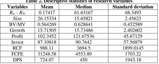
Table 2 representsthe descriptive statistics for research variables.
Table 2. Descriptive statistics of research variables
Variables Mean Median Standard deviation
Rit - RFt 0.17417 61.63167 68.3493
Size 26.15334 15.65821 2.45623
BV/MV 0.564269 0.628641 0.452589
Growth 15.71505 15.73486 2.402602
Profit 102.3452 121.67536 45.67129
Invest 87.10818 90.7642 57.56879
RCF 988.11 3694.5 1899.0145
FCFE 31248.58 4553.89 1703.22
DPS 724.07 450 1943.18
Table 3. Stationary test of research variables Variable Levin, Lin and Chu test
Statistic value Significance level
Rit - RFt -52.75 0.000
Size -45.32 0.000
BV/MV -20.31 0.000
Growth -26.03 0.000
Profit -32.72 0.000
Invest -24.39 0.000
RCF -45.13 0.000
FCFF -43.19 0.000
DPS -32.27 0.000
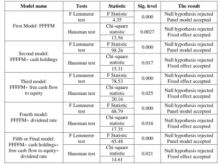
F Lemmer test used to determine which one of the pooled or panel models is appropriate for estimation. The results are as Table 4.
Table 4. F Lemmerer and Hausman tests for the models
Model name Tests Statistic Sig. level The result
First Model: FFFFM
F Lemmerer test
F Statistic
0.000 Null hypothesis rejected Panel model accepted 4.35
Hausman test
Chi-square
statistic 0.0027 Null hypothesis rejected Fixed effect accepted 13.56
Second model: FFFFM+ cash holdings
F Lemmerer test
F Statistic
0.000 Null hypothesis rejected Panel model accepted 98.26
Hausman test
Chi-square
statistic 0.017 Null hypothesis rejected Fixed effect accepted 15.31
Third model: FFFFM+ free cash flow
to equity
F Lemmerer test
F Statistic
0.000 Null hypothesis rejected Fixed effect accepted 78.53
Hausman test
Chi-square
statistic 0.025 Null hypothesis rejected Fixed effect accepted 20.16
Fourth model: FFFFM+ dividend rate
F Lemmerer test
F Statistic
0.000 Null hypothesis rejected Panel model accepted 68.79
Hausman test
Chi-square
statistic 0.016 Null hypothesis rejected Fixed effect accepted 17.35
Fifth or Final model: FFFFM+ cash holdings+ free cash flow to equity+
dividend rate
F Lemmerer test
F Statistic
0.000 Null hypothesis rejected Panel model accepted 65.48
Hausman test
Chi-square
statistic 0.021 Null hypothesis rejected Fixed effect accepted 14.61
null hypothesis rejects; and the panel method with fixed effects is used to estimate the regression model.
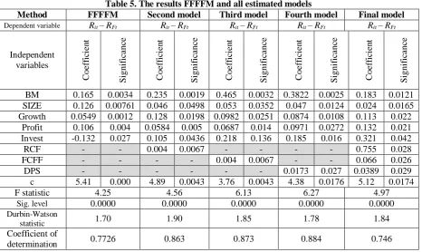
The results of calculations for the models are as Table 5.
Table 5. The results FFFFM and all estimated models
Method FFFFM Second model Third model Fourth model Final model
Dependent variable Rit – RFt Rit – RFt Rit – RFt Rit – RFt Rit – RFt
Independent variables Coe ff ic ie n t S igni fi ca nc e Coe ff ic ie n t S igni fi ca nc e Coe ff ic ie n t S igni fi ca nc e Coe ff ic ie n t S igni fi ca nc e Coe ff ic ie n t S igni fi ca nc e
BM 0.165 0.0034 0.235 0.0019 0.465 0.0032 0.3822 0.0025 0.183 0.0121 SIZE 0.126 0.00761 0.046 0.0498 0.053 0.0352 0.047 0.0124 0.024 0.0165 Growth 0.0549 0.0012 0.128 0.0198 0.0982 0.0251 0.0874 0.0108 0.113 0.022
Profit 0.106 0.004 0.0584 0.005 0.0687 0.014 0.0971 0.0272 0.132 0.021 Invest -0.132 0.027 0.105 0.0436 0.218 0.136 0.185 0.016 0.321 0.042
RCF - - 0.004 0.0067 - - - - 0.755 0.028
FCFF - - - - 0.004 0.0067 - - 0.066 0.026
DPS - - - 0.0173 0.027 0.0389 0.029
c 5.41 0.000 4.89 0.0043 3.76 0.0043 4.38 0.0176 5.12 0.0174
F statistic 4.25 4.56 6.13 6.27 4.97
Sig. level 0.0000 0.0000 0.0000 0.0000 0.0000
Durbin-Watson
statistic 1.70 1.90 1.85 1.78 1.84
Coefficient of
determination 0.7726 0.863 0.873 0.884 0.746
According to Table 5, the significance of F-statistic for the model is less than 0.05, which means there is a significant linear relation between independent and dependent variables in this model.
Durbin-Watson test investigates the independence of errors. The lack of correlation between errors is accepted if Watson statistic is close to two. According to Table 5, Durbin-Watson statistic is proper for all models. Therefore, all variables have significant relationships according to results of estimated FFFFM.
In Table 5, primary FFFFM has a coefficient of determination 0.7726 and among the studied variables, only the investment variable has a negative relationship, but the other variables have positive relationships.
According to the results in Table 5, the second estimated model has a coefficient of determination 0.863. Also all studied variables have shown significant positive relationships. The investment variable also indicates a positive and significant effect after adding the cash holdings to FFFFM. This result indicates that adding cash holding variable improves the predict power of return prediction in TSE and outperforms primary FFFFM.
The results of third estimated model with a coefficient of determination 0.873 imply that except for the investment variable, which is insignificant, other variables have positive significant relationship. This model also outperforms both the primary FFFFM and second model.
The fourth estimated model with a coefficient of determination 0.884 is the most powerful model in predicting return in TSE. It outperforms FFFFM and all other estimated models. The results show significant and positive relationship for all variables.
market value, company size, growth opportunities, profitability and investment, cash holdings, dividend, and free cash flow to equity).
In this research, in order to improve the prediction of stock returns, along with the FFFFM, four new regression models developed based on the basic FFFFM model. First new regression model was made by the combination of the FFFFM and the cash holdings variable (FFFFM+ cash holdings). The second new regression model created by the combination of the FFFFM and the free cash flow to equity variable (FFFFM+ free cash flow to equity). The third new regression model designed by the combination of the FFFFM and the dividend rate variable (FFFFM+ dividend rate). Finally, the forth-new regression model formulated by the combination of the FFFFM and all corporate feature variables (FFFFM+ cash holdings variable+ free cash flow to equity+ dividend rate). In the next step, the predictive power of the models compared.
The findings indicate that the coefficient of determinations (R2) for the five regression models are 0.7726, 0.863, 0.876, 0.884, and 0.746, respectively. In other words, the predictive power of the models are different. However, the order of models in terms of their predictive power is fourth> third>second>first>fifth. It means that the fourth model that creates more accurate and closer-to-reality predictions for stock returns in Tehran Stock Exchange is the best and the fifth model is the worst.
5. Conclusion
Given the impact of stock returns on shareholders' decisions, the researchers need to examine factors influencing the stock returns. This research investigates the effects of three important corporate variables on the primary FFFFM in TSE. In addition, it examines the improvement in the accuracy of predicting the returns by developing four new regression models based on primary FFFFM. The models estimated through panel data regression with fixed effects. According to the results, all five variables in FFFFM (i.e. book to market value ratios, firm size, growth opportunity, profitability, and investment) and corporate feature variables (cash holdings, dividend, and free cash flow to equity) has positive and significant relation to the returns. In addition, the predict power of returns improves when corporate feature variables adds to FFFFM. Generally speaking, according to the results, intelligent selection of variables and including them FFFFM significantly improves the predictive power, however the inclusion of all variables without intelligent review of the literature and roughly selection variables could not outperform traditional FFFFM.
Comparing the coefficient of determinations (R2) of the models indicate that the fourth model (FFFFM+ dividend rate) creates more accurate and closer-to-reality predictions for stock returns in Tehran Stock Exchange and that it is the best and the fifth model is the worst.
References
Aharoni, G., Grundy, B., and Zeng, Q., (2013). "Stock returns and the Miller Modigliani valuation formula: Revisiting the Fama French Analysis", Journal of Financial Economics, Vol. 110, No. 2, pp. 347-357.
Cakici, N., (2015). The Five-factor Fama-French Model: International Evidence. Available at SSRN: https://ssrn.com/abstract=2601662 or http://dx.doi.org/ 10.2139/ ssrn.2601662.
Fama, E.F., and French, K.R., (1993). "Common risk factors in the returns on stocks and bonds",
Journal of Financial Economics, Vol. 33, No. 1, pp. 3–56.
Fama, E.F., and French, K.R., (2016). "Dissecting anomalies with a five-factor model", Review of Financial Studies, Vol. 29, No. 1, pp. 69-103.
Fama, E.F., and French, K.R., (2016b). International tests of a five-factor model, manuscript, Tuck School of Business, Dartmouth College.
Hausman, J.A. (1978). "Specification tests in econometrics", Econometrica, Vol. 46, No. 6, pp. 1251– 1271.
Lintner, J., (1965). "The valuation of risk assets and the selection of risky investment in stock portfolios and capital budgets", The Review of Economics and Statistics, Vol. 47, No. 1, pp. 13-37.
Maxim, Caudia A., (2015). "The evaluation of CAPM, Fama-French and APT models on the Romanian capital market", Applied Financial Research, pp. 1-10.
Miller M.H., and Modigliani, F., (1961). "Dividend policy, growth, and the valuation of shares", The Journal of Business, Vol. 34, No. 4, pp. 411-4.
Novy, R., Marx, L., and Alan S., (2013). "The other side of value: The gross profitability premium",
Journal of Financial Economics, Vol. 108, No. 1, pp. 1-28.
Racicot, F., and Theoret, R., (2015). "The q-factor model and the redundancy of the value factor: An application to hedge fund: A portfolio manager and investor’s perspective", Alternative Investment Analyst Review (CAIA), Vol. 3, No. 4, pp. 52–64.
Sharpe, W.F., (1964). "Capital asset prices: A theory of market equilibrium under conditions of risk",
Journal of Finance, Vol. 19, No. 3, pp. 425-42.
Treynor, J. L., (1962). Toward a theory of market value of risky assets. (Unpublished manuscript). Final version in Asset Pricing and Portfolio Performance (pp. 15-22), 1999, Robert A. Korajczyk (Ed.). London: Risk Books.
This article can be cited: Rowshandel, SH., Anvary Rostamy, A.A., Noravesh, I., Darabi, R., (2019). "Developing revised Fama-French Five-Factor models by including dividend rate, cash holdings, and free cash flow to equity: evidence of Tehran stock exchange", Journal of Industrial Engineering and Management Studies, Vol. 6, No. 1, pp. 68-78.