CRL 96 2 pdf

Characterization of Errors in

Compositing Panoramic Images

Sing Bing Kang and Richard Weiss

Digital Equipment Corporation

Cambridge Research Lab

Digital Equipment Corporation has four research facilities: the Network Systems Laboratory, the Systems Research Center, and the Western Research Laboratory, all in Palo Alto, California; and the Cambridge Research Laboratory, in Cambridge, Massachusetts.

The Cambridge laboratory became operational in 1988 and is located at One Kendall Square, near MIT. CRL engages in computing research to extend the state of the computing art in areas likely to be important to Digital and its customers in future years. CRL’s main focus is applications technology; that is, the creation of knowledge and tools useful for the preparation of important classes of applications.

CRL Technical Reports can be ordered by electronic mail. To receive instructions, send a mes-sage to one of the following addresses, with the word help in the Subject line:

On Digital’s EASYnet: CRL::TECHREPORTS On the Internet: [email protected]

This work may not be copied or reproduced for any commercial purpose. Permission to copy without payment is granted for non-profit educational and research purposes provided all such copies include a notice that such copy-ing is by permission of the Cambridge Research Lab of Digital Equipment Corporation, an acknowledgment of the authors to the work, and all applicable portions of the copyright notice.

The Digital logo is a trademark of Digital Equipment Corporation.

Cambridge Research Laboratory One Kendall Square

Cambridge, Massachusetts 02139

Characterization of Errors in

Compositing Panoramic Images

Sing Bing Kang and Richard Weiss

Digital Equipment Corporation

Cambridge Research Lab

CRL 96/2 June, 1996

Abstract

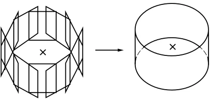
A panoramic image has 360 horizontal field of view, and it can provide the viewer the impres-sion of being immersed in the scene to a certain extent. A panorama is created by first taking a sequence of images while rotating the camera about a vertical axis. These images are then projected onto a cylindrical surface before being seamlessly composited. The cross-sectional circumference of the cylindrical panorama is called the compositing length.

This work characterizes the error in compositing panoramic images due to errors in intrinsic camera parameters. The intrinsic camera parameters that are considered are the camera focal length and the radial distortion coefficient. We show that the error in the compositing length is

more sensitive to the error in the camera focal length. Especially important is the discovery that the relative error in compositing length is always smaller than the relative error in the focal length. This means that the error in focal length can be corrected by iteratively using the composited length to compute a new and more correct focal length. This compositing approach to camera calibration has the advantages of not requiring both feature detection and separate prior calibration.

Keywords: 3-D scene modeling, image compositing, camera calibration.

c Digital Equipment Corporation 1996. All rights reserved.

1

Contents i

Contents

1 Introduction: : : : : : : : : : : : : : : : : : : : : : : : : : : : : : : : : : : : : : : 1 1.1 Analyzing the error in compositing length . . . 1 1.2 Camera calibration . . . 1 1.3 Motivation and outline . . . 2

2 Generating a panoramic image : : : : : : : : : : : : : : : : : : : : : : : : : : : : 3

3 Compositing errors due to misestimation of focal length : : : : : : : : : : : : : : : 4 3.1 Derivation . . . 5 3.2 Image compositing approach to camera calibration . . . 10

4 Compositing errors due to misestimation of radial distortion coefficient : : : : : : 14

5 Effect of error in focal length and radial distortion coefficient on 3-D data : : : : : 18

ii LIST OF FIGURES

List of Figures

1 Compositing multiple rotated camera views into a panorama. The ’’ marks

indi-cate the locations of the camera optical and rotation center. . . 3

2 Effect of inexact focal length: (a) actual mapping from second cylindrical image; (b) theoretical displacement; (c) actual mapping to first cylindrical image. See text. 6 3 Graph of error in displacement vs. pixel location for varying estimated focal length f. f tr ue =274:5N =50andl=232. . . 7

4 Graph of error in displacement vs. pixel location for varying number of framesN. f tr ue =274:5f =294:5andl =232. . . 8

5 Overlap between successive imagesI k ;1 and Ik, with centers at O k ;1 and O k re-spectively. . . 9

6 Graph of estimated focal length vs. number of iteration. f0 is the initial estimated focal length; the actual focal length is 274.5. The solid lines represent actual values whereas dashed lines represent predicted values. . . 12

7 Example undistorted image sequence of synthetic room. . . 13

8 Panorama of synthetic room after compositing the sequence in Figure 7. . . 13

9 Panorama of synthetic room corresponding to an erroneous focal length. . . 13

10 Panorama of synthetic room corresponding to an erroneous focal length, but using a simple weighted compositing technique. . . 14

11 Mapping of pixels from the second cylindrical image to the first. The transfor-mationf indicates mapping from cylindrical to rectilinear coordinates with focal lengthf while transformationindicates the radial distortion mapping with radial distortion factor . Terms with the subscript “true” represent the correct entities while those without this subscript represent estimated ones. Rect0 is the undis-torted rectilinear image. See text. . . 15

12 Graph of equivalent focal length error vs. error in, the radial distortion factor. The true focal length (f tr ue) is 274.5 and the true radial distortion factor ( tr ue) is 2:810 ;7 . . . 16

LIST OF FIGURES iii

14 Panorama of synthetic room (same camera location as in Figure 13) corresponding to an erroneous focal length. . . 17 15 Variation of compositing length error vs. errors in both focal length and radial

distortion coefficient. The deviations are all in terms of percentages. The nominal focal length and radial distortion coefficient are 274.5 and2:810

;7

respectively.

See text for descriptions ofdL0anddL1. . . 18 16 Example recovered 3-D data (corresponding to the correct focal length of 274.5). . 19 17 Graph of RMS 3D error of recovered stereo data vs. estimated focal length. The

true focal length is 274.5 (indicated by the vertical dashed line). . . 20 18 Graph of RMS 3D error of recovered stereo data vs. error in radial distortion

coefficient. Typical real values of is of the order of10 ;7

. The zero error in

1 Introduction 1

1

Introduction

A panoramic image has a 360 horizontal field of view. Panoramic images of scenes have interest-ing applications in computer vision and visualization, since they are able to provide the viewer the

impression of being immersed in the scene to a certain extent. For example, Apple’s QuickTime VRTM

[Chen, 1995] product uses panoramas for scene visualization. In computer vision, applying the stereo algorithm on multiple panoramas allows the entire 3D scene data points to be extracted [Kang and Szeliski, 1995] and subsequently modeled [Kang et al., 1995].

A panoramic image is produced by following a series of steps: First, a sequence of images is taken while rotating a camera about a vertical axis that passes through the camera optical center. Each image in the sequence is then projected onto a cylindrical surface whose cross-sectional radius is an initially estimated focal length (see Figure 1). The panoramic image is subsequently created by determining the relative displacements between adjacent images in the sequence and

compositing the displaced sequence of images. The length of the panoramic image is termed the

compositing length.

1.1

Analyzing the error in compositing length

In this technical report, we describe the effect of errors in intrinsic camera parameters on the compositing length. We are not aware of any prior work in this specific area. In particular, we consider the focal length and the radial distortion coefficient. An important consequence of this analysis is that a much better estimate of the camera focal length can be calculated from the current compositing length. Hence by iterating the process of projecting onto a cylindrical surface (whose cross-sectional radius is the latest estimation of the camera focal length) and compositing the new sequences, we quickly arrive at the camera focal length within a specified error tolerance. We show later that the convergence towards the true focal length is exponential. This method constitutes a simple means of calibrating a camera.

1.2

Camera calibration

2 1 Introduction

roundness of spheres [Penna, 1991; Stein, 1995], straightness of lines [Brown, 1971; Stein, 1995]). We propose a method for featureless camera calibration based on an iterative scheme of projecting rectilinear images to cylindrical images and then compositing. In addition to determining the camera focal length, this technique results in a panoramic image (i.e., with 360 horizontal field of view) that is both physically correct (ignoring radial distortion effects) and seamlessly blended.

The basis of the compositing approach to camera calibration is the discovery that the relative compositing length error due to camera focal length error is disproportionately much less (i.e., in terms of percentages) than the relative focal length error. When a planar image is projected to a cylinder as in the compositing process, mis-estimation of the radius of the cylinder will produce an erroneous warping of the image that will affect the length of the final composite image. However, it turns out that near the center of the overlap between successive images, the amount of combined warping for both images is minimal and so is the effect of the mis-estimation. The result of this is that the percent error in length of the composite image is less than the percent error in the focal length. This makes it possible to use the composite length to recover a better estimate of the camera

focal length.

The proposed technique has the advantage of not having to know the camera focal length when a panorama is to be generated from a sequence of images. This is in contrast to Apple’s QuickTime VRTM

[Chen, 1995], which we believe that a reasonably good estimate of camera focal length is required a priori. This is also the case for McMillan and Bishop’s method of creating panoramas

[McMillan and Bishop, 1995]. Their method of estimating the camera focal length necessitates small panning rotations and relies on translation estimates near the image centers.

The method of calibration that is closest to ours is that of Stein’s [Stein, 1995], in which features are tracked throughout the image sequence taken while the camera is rotated a full 360 . While this technique results in accurate camera parameters, it still requires feature detection and tracking. Our technique directly uses the given image sequence of the scene to determine camera focal length without relying on specific tracked features.

1.3

Motivation and outline

2 Generating a panoramic image 3

Figure 1: Compositing multiple rotated camera views into a panorama. The ’’ marks indicate the locations of the camera optical and rotation center.

to take stereo snapshots of the scene at various poses and then merge these 3-D stereo depth maps. This is not only computationally intensive, but the resulting merged depth maps may be subject to merging errors, especially if the relative poses between depth maps are not known exactly. The 3-D data may also have to be resampled before merging, which adds additional complexity and potential sources of errors.

The outline of this technical report is as follows: Section 2 reviews how a panoramic image is produced from a set of images. This is followed by section 3 which gives a detailed analysis of the compositing error due error in the camera focal length in Section 3. A consequence of this analysis is the iterative compositing approach to camera calibration. Section 4 looks at the effect of mises-timating the radial distortion coefficient on the panoramic compositing length. We then describe the effect of errors in both focal length and radial distortion coefficient on the reconstructed 3-D data in section 5 before summarizing in section 6.

2

Generating a panoramic image

A panoramic image is created by compositing a series of rotated camera image images, as shown in Figure 1. In order to create this panoramic image, we first have to ensure that the camera is rotating about an axis passing through its optical center, i.e., we must eliminate motion parallax when panning the camera around. To achieve this, we manually adjust the position of camera relative to an X-Y precision stage (mounted on the tripod) such that the motion parallax effect disappears when the camera is rotated back and forth about the vertical axis [Stein, 1995].

4 3 Compositing errors due to misestimation of focal length

parameters, namely , the radial distortion coefficient, and f, the camera focal length. This is accomplished by taking snapshots of a calibration dot grid pattern at known spacings and using the iterative least squares algorithm described in [Szeliski and Kang, 1994]. As a result of our analysis reported here, this calibration step can be skipped if the radial distortion coefficient is insignificant.

A panoramic image is created using the following steps [Kang and Szeliski, 1995]:

1. Capture a sequence of rotated camera views about a vertical axis passing through the camera optical center;

2. Undistort the sequence to correct for;

3. Warp the undistorted (rectilinear) sequence to produce a corresponding cylindrical-based image sequence whose cross-sectional radius is equal to the camera focal length f; and finally

4. Composite the sequence of images [Szeliski, 1994].

The compositing technique comprises two steps: rough alignment using phase correlation, and iterative local refinement to minimize overlap intensity difference between successive images. In both steps, the translation is assumed to be in one direction only, namely in the x-direction (since the cylindrical-based images have been “flattened” or unrolled). This is a perfectly legitimate

assumption, since camera motion has been constrained to rotate about a vertical axis during image sequence capture. If the estimated focal length is exact, then the error in the composited length is due to the digitization and image resampling effects, the limit in the number of iterations during local matching, and computer truncation or rounding off effects.

The rough alignment step has been made more robust by adding the iterative step of checking the displacement corresponding to the peak—if the intensity RMS error in matching the overlap regions is high, the peak is tagged as false and the next highest peak is chosen instead.

3

Compositing errors due to misestimation of focal length

3.1 Derivation 5

used, sayf

tr ue, then the expected length of the composited panoramic image 1

is

L=2f

tr ue (1)

If the focal lengthf used is incorrect, then the mapped cylindrical images are no longer phys-ically correct. The compositing step will attempt to minimize the error in the overlap region of successive images, but there is still a net error in compositing lengthL.

Since each column in a rectilinear image is projected to another column in the cylindrical image and translation is constrained to be along the x-direction, it suffices to consider only a scanline in our analysis. We assume for simplicity that the images are “fully textured” so that matching between corresponding pixels is unambiguous. We also assume, for ease of analysis, that the amount of camera rotation between successive frames is the same throughout the sequence (this need not be so in practice). In our analysis, the net translation is computed by minimizing

the sum of squares of the pixel displacements from their matching locations. In other words, even after translation with interpolation, the pixels in the second image will not match the pixels in the first image at the same location. Each pixel will match one at a displaced location. The translation which minimizes the sum of their squares is the one that results in zero average displacement.

3.1

Derivation

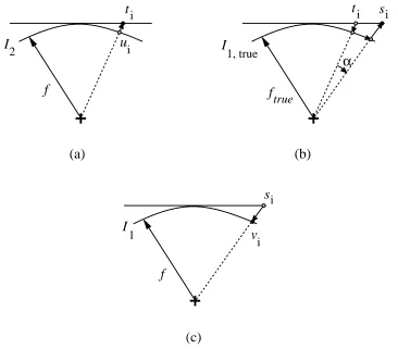
In order to model the displacement of each pixel u

i in the second cylindrical image, we map it back tot

i in the image plane, find the corresponding pixel s

i in the first image based on the actual rotation, and map that back to v

i in the cylindrical image. This is illustrated in Fig. 2, where I

1 and I

2 are the first and second cylindrical images, respectively. I

1tr ue is the true cylindrical first image whileis the amount of actual camera rotation between successive frames, i.e.,2=N,

N being the number of images in the sequence. Recall that the cylindrical images are formed by warping the images into a cylindrical surface whose cross-sectional radius is the estimated focal length. The mappings are given by the following equations:

t i

= ftan u

i f

!

1

In creating the panoramic image, the order of compositing isI 1,

I 2, ...,

I N;1,

I N,

I

1, where I

kis the

kth image in the sequence andN is the number of images in the sequence. The compositing lengthLis actually the displacement of the first frameI

6 3 Compositing errors due to misestimation of focal length u_i true 1, true f I f I₂ 1 f I α v i s_i t_i t_i s_i (a) (b) (c)

Figure 2: Effect of inexact focal length: (a) actual mapping from second cylindrical image; (b) theoretical displacement; (c) actual mapping to first cylindrical image. See text.

s i = f tr ue tan tan ;1 t i f tr ue ! + ! (2) v i

= ftan ;1

s i f

!

As before, = 2=N andf

tr ue is the correct focal length while

f is the estimated focal length used.

Using MathematicaTM

[Wolfram, 1991], we find that, up to the third order inu iand , v i (u i

) = u i + f 2 f 2 tr ue +f 2 u 2 i ;f 2 tr ue u 2 i f 2 f tr ue +

(f ;f tr ue

3.1 Derivation 7

−120 −80 −40 0 40 80 120

Pixel position (u)

−1.2 −0.8 −0.4 0.0 0.4 0.8

Error in displacement (pixels)

f = 254.5

f = 264.5

f = 274.5

f = 284.5

f = 294.5

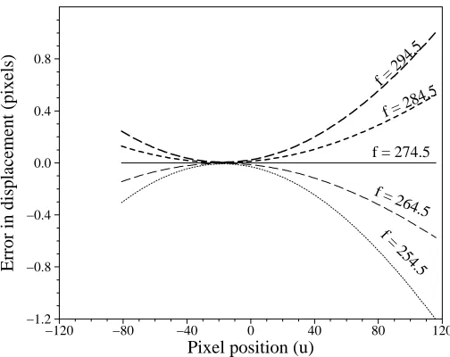
Figure 3: Graph of error in displacement vs. pixel location for varying estimated focal lengthf.

f tr ue

=274:5N =50andl=232.

+

(f ;f tr ue

)(f +f tr ue )(f 2 f 2 tr ue +4f 2 u 2 i ;6f 2 tr ue u 2 i ) 3f 4 f tr ue 3 (3)

The displacement between two successive frames atu i is

d i

(u i

) =v i

(u i

);u

i; the plot of the variation ofd

i (u

i

)versus u i for

f tr ue

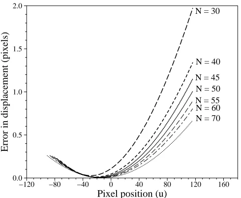
= 274:5and N = 50 for different values of misestimated values of f is shown in Fig. 3. It is interesting to note that the minimum displacement due to focal length error occurs near the center of the overlap. The change in the displacement error distribution due to the amount of overlap (changing number of framesN) is shown in Fig. 4. As can be observed, as N increases, the amount of overlap increases, and interestingly enough, the overall error decreases. If all are kept constant except for the image lengthl, the error distribution remains the same save foru

1 and u

2, the two end pixel locations of the overlap area. They shrink to decrease the amount of horizontal overlap asldecreases. The mean displacement between two successive frames (see Fig. 5) is

D= P u 2 u i =u 1 (v i (u i );u

i ) u 2 ;u 1 +1 (4)

Note that if the interframe displacement is equal throughout the sequence and that the length of each image isl, thenu

2

= l =2andu 1

= 2f tr ue

8 3 Compositing errors due to misestimation of focal length

−120 −80 −40 0 40 80 120 160

Pixel position (u)

0.0 0.5 1.0 1.5 2.0

Error in displacement (pixels)

N = 30

N = 40

N = 45 N = 50 N = 55 N = 60 N = 70

Figure 4: Graph of error in displacement vs. pixel location for varying number of frames N.

f tr ue

=274:5f =294:5andl=232.

composite length, is given by

L=N

D (5)

Suppose we reestimate the focal length from the composite length, namelyf 0

=L=(2). The question is: Isf

0

a better estimate of the focal length thanf? It turns out that for initial estimates off close to the true value, the answer can be shown to be yes. To see this, iff f

tr ue, then from (3), (4) and (5), we get

f 0 = L 2 N 2 (" f tr ue

+ 1; f 2 tr ue f 2 ! u 2 f tr ue # + " 1; f 2 tr ue f 2 ! u; 1 3 1; f 2 tr ue f 2 ! 5 f 2 tr ue f 2 ;3 ! u 3 f 2 tr ue # 2 + " 1 3 f tr ue 1; f 2 tr ue f 2 !

;2 1; f 2 tr ue f 2 ! f 2 tr ue f 2 ; 2 3 ! u 2 f tr ue # 3 ) f tr ue

3.1 Derivation 9 I k k-1 I overlap area O k k-1 O 1 u 2 u

Figure 5: Overlap between successive images I

k ;1 and I

k, with centers at O

k ;1 and O k respec-tively. + " 1; f 2 tr ue f 2 ! u; 1 3 1; f 2 tr ue f 2 ! 5 f 2 tr ue f 2 ;3 ! u 3 f 2 tr ue # + " 1 3 f tr ue 1; f 2 tr ue f 2 !

;2 1; f 2 tr ue f 2 ! f 2 tr ue f 2 ; 2 3 ! u 2 f tr ue # 2 (6)

noting that=2=N, and where

u = P u 2 i=u 1 i u 2 ;u 1 +1 = 1 2 (u 2 +u 1 )= f tr ue N (7) u 2 = P u 2 i=u1 i 2 u 2 ;u 1 +1 = 1 3 u 2 2 +u 1 u 2 +u 2 1 + 1 2 (u 2 ;u 1 ) = 1 3 (u 2 +u 1 ) 2 ;u 2 u 1 + 1 2 (u 2 ;u 1 ) = 1 3 " 4 2 f 2 tr ue N 2 ; 2f tr ue N ; l 2 ! l 2 + f tr ue N ; l 2 # (8) and u 3 = P u2 i=u 1 i 3

10 3 Compositing errors due to misestimation of focal length = 1 4 (u 2 +u 1 ) u 2 2 +u 2 1 +u 2 ;u 1 = 1 2 f tr ue N 2 4 2f tr ue N ; l 2 ! 2 + l 2 4 + 2f tr ue N ;l 3 5 (9) Hence f tr ue ;f 0 ( u 2 f tr ue + " u; 1 3 5 f 2 tr ue f 2 ;3 ! u 3 f 2 tr ue # + " f tr ue 3 ;2 f 2 tr ue f 2 ; 2 3 ! u 2 f tr ue # 2 ) f 2 tr ue f 2 ;1 ! f tr ue f f tr ue +f 2f 2 ( u 2 f 2 tr ue + u f tr ue ; 2 3 u 3 f 3 tr ue ! + 1 3 ; 2 3 u 2 f 2 tr ue ! 2 ) (f tr ue ;f) 2 ( u 2 f 2 tr ue + u f tr ue ; 2 3 u 3 f 3 tr ue ! + 1 3

1;2 u 2 f 2 tr ue ! 2 ) (f tr ue

;f) (10)

Let 1 = u f tr ue = N (11) 2 = u 2 f 2 tr ue = 1 3 " 4 2 N 2 ; 2 N ; l 2f tr ue ! l 2f tr ue + 1 f tr ue N ; l 2f tr ue !# (12) and 3 = u 3 f 3 tr ue = 1 2 N 2 4 2 N ; l 2f tr ue ! 2 + l 2f tr ue ! 2 + 2 f tr ue N ; l 2f tr ue ! 3 5 (13)

Thus (10) becomes

f tr ue ;f 0 2 2 + 1 ; 2 3 3 + 1 3

(1;2 2 ) 2 (f tr ue

;f)=(f tr ue

;f) (14) IfN is large, which is typical (in practice, N is about 50), thenjf

tr ue ;f

0 j jf

tr ue

;fj. This implies that the estimated focal length based on the composited length is a significantly better estimate.

3.2

Image compositing approach to camera calibration

The previous result suggests a direct, iterative method of simultaneously determining the camera focal length and constructing a panoramic image. This iterative image compositing approach to

camera calibration has the advantages of not requiring both feature detection and separate prior

3.2 Image compositing approach to camera calibration 11

Let the initial estimate of focal length be f 0. Determine compositing length L

0 from f

0. Set k =1.

1. Calculate f k

=L k ;1

=(2).

2. Determine compositing length L

k from f

k. 3. If (jL

k ;L

k ;1

j) f kk+1

Go to Step 1.

g else

f

k is the final estimated focal length.

Since we know that the iterated value of f

k converges toward f

tr ue, it would be interesting to determine its rate of convergence. (14) can be rewritten as a recurrence equation (assuming equality rather than approximation)

f tr ue

;f k

=(f tr ue

;f k ;1

) (15)

Rearranging, we have

f k

;f k ;1

=(1;)f tr ue

(16)

from which the solution can be found to be

f k

=f tr ue

+(f 0

;f tr ue

) k

(17)

Hence, the convergence off

k towards f

tr ue is exponential in the vicinity of the true focal length, as shown by (17). This also indicates that the convergence is faster if the number of frames N increases, the image lengthldecreases, or the true focal lengthf

tr ueincreases. As an example, for N =50,l =232, andf

tr ue

=274:5,=0:117.

The graph in Figure 6 shows the convergence of estimated focal length from different initial estimates. (A sequence of the synthetic room is shown in Figure 7 and the corresponding compos-ited image is shown in Figure 8.) It is interesting to note that the actual estimated focal lengths are

smaller than theoretically predicted ones. One of the reasons could be due to effects of resampling

12 3 Compositing errors due to misestimation of focal length

0 1 2 3

Number of iterations

250 260 270 280 290 300

Focal length

actual predicted f0 = 294

f0 = 284

f0 = 274.5

f0 = 264

f0 = 254

Figure 6: Graph of estimated focal length vs. number of iteration. f0 is the initial estimated focal length; the actual focal length is 274.5. The solid lines represent actual values whereas dashed lines represent predicted values.

textured,” which is difficult to realize in practice and even in simulations. Finally, shifts greater than 1 pixel are not likely to influence the net shift correctly.

A panorama of the synthetic room is shown in Figure 9. As can be seen, the effect of misesti-mating the focal length in compositing is a blurring effect, presumably about the correct locations. When a rectilinear image is projected onto a cylindrical surface of the wrong cross-sectional

ra-dius, which is also the estimated focal length, the error in pixel placement increases away from the central image column. Having many cylindrical-converted images superimposed would thus have the effect of locally smearing the correct locations. This suggests that a good scheme of composit-ing many images to form a panorama is to down-weight the pixels away from the central image column during compositing. Indeed, Figure 10 shows the effect of using such a simple scheme. Here each pixel is weighted by a factor proportional tojc;c

center j

, wherecis the current pixel column,c

center the central pixel column, and

3.2 Image compositing approach to camera calibration 13

Image 1 Image 2 Image (N-1) Image N

Figure 7: Example undistorted image sequence of synthetic room.

Figure 8: Panorama of synthetic room after compositing the sequence in Figure 7.

To further illustrate the robustness of this approach, we have also started the iterative process

with the original rectilinear images, (i.e., f 0

= 1), which would be the worst case focal length initialization. The convergence of the focal length value is: 1 ! 281:18 ! 274:40 ! 274:24. As before, the actual focal length is 274.5. The process arrives at virtually the correct focal length in just two iterations. This result is very significant; it illustrates that in principal, we can start without a focal length estimate.

14 4 Compositing errors due to misestimation of radial distortion coefficient

Figure 10: Panorama of synthetic room corresponding to an erroneous focal length, but using a simple weighted compositing technique.

4

Compositing errors due to misestimation of radial distortion

coefficient

Another important camera intrinsic parameter that could cause errors in the compositing length is the radial lens distortion. If (x

u y

u

) is the undistorted image location and(x d

y d

) is its radially distorted counterpart, then

x u = x d (1+ 1 r 2 d + 2 r 4 d +:::) y u = y d (1+ 1 r 2 d + 2 r 4 d

+:::) (18)

where r d = q x 2 d +y 2 d

For our work, we use only the first radial coefficient term=1:

x u

= x d

(1+r 2 d ) y u = y d

(1+r 2 d

) (19)

with the inverse

x d

= x

u 1+r

2 d y d = y u 1+r

4 Compositing errors due to misestimation of radial distortion coefficient 15

κ_true

Cyl₁

Rect’₂

Rect₁

Rect0₁

Rect’₁

Cyl_2,true Cyl_1,true

Rect0₂

Rect₂

Cyl

2

κ f

true

f -1

-1

-1 -1

α rotate

by f

κ

κ_true f

true

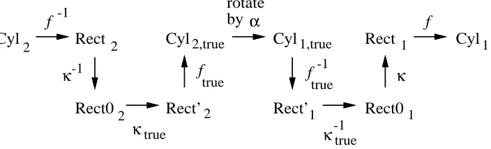
Figure 11: Mapping of pixels from the second cylindrical image to the first. The transformation

f indicates mapping from cylindrical to rectilinear coordinates with focal length f while trans-formationindicates the radial distortion mapping with radial distortion factor. Terms with the subscript “true” represent the correct entities while those without this subscript represent estimated ones. Rect0 is the undistorted rectilinear image. See text.

+

1

9 r

1 27

3 +

r 2 u 2 2

2 ;

1 729

6 +

1 27

3 +

r 2 u 2 2

!1 3

2 ;

2 3

(21)

(21) is found using MathematicaTM

[Wolfram, 1991]. Details of lens distortion modeling can be found in [Slama, 1980].

The transformations required to show the effect of incorrect focal length and radial distortion coefficient are depicted in Figure 11. We assume that the cylindrical images are displaced by an angular amount . To see how these transformations come about, consider the right half of the series of transformations beyond “rotate by .” We require the mapping from the correct cylindrical image point to the actual cylindrical image point, given estimates of f and . To generate the correct undistorted rectilinear image, we have to unproject from the cylindrical surface to the flat rectilinear surface (f

;1

tr ue) and then radially undistort ( ;1

16 4 Compositing errors due to misestimation of radial distortion coefficient

−1.0e−06 −5.0e−07 0.0e+00 5.0e−07 1.0e−06

k_est − k_true −2.0

−1.0 0.0 1.0 2.0

f_est − f_true

predicted

actual

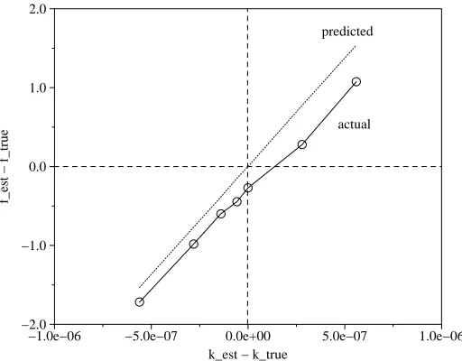
Figure 12: Graph of equivalent focal length error vs. error in, the radial distortion factor. The true focal length (ftr ue) is 274.5 and the true radial distortion factor (tr ue) is2:810

;7 .

image center row, the average displacement in y is zero.

The effect of misestimating the radial distortion coefficientfor a typical value off =274:5 and = 2:8 10

;7

is shown in Figure 12. As can be seen, the effect is almost linear, and despite significant errors in, the resulting error in the effective focal length is small (<1%). This illustrates that for typical real focal lengths and radial distortion coefficients, the dominant factor in the compositing length error is the accuracy of the focal length.

The appearance of the panorama due to error in radial distortion coefficientis not very per-ceptible if the radial distortion is typically small (of the order of 10

;7

). An extreme case that corresponds to a large error in radial distortion coefficient (by 10

;5

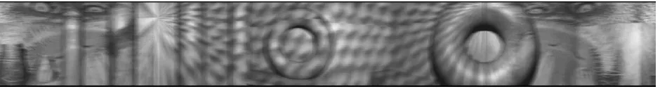
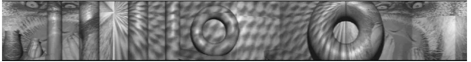
) can be seen in Figure 13. Here, a simple scheme of compositing by direct averaging is performed, and there is a perceptible ghosting effect. However, using the weighted compositing scheme results in a much sharper im-age, as shown in Figure 14. There is still some blurring effects, which is more pronounced away from the central horizontal row of the panorama, but this is to be expected with errors in.

4 Compositing errors due to misestimation of radial distortion coefficient 17

Figure 13: Another panorama of synthetic room corresponding to a large erroneous radial distor-tion coefficient (by1:010

;5 ).

Figure 14: Panorama of synthetic room (same camera location as in Figure 13) corresponding to an erroneous focal length.

between the correct compositing length and expected compositing length. The first error (dL0) measures the consistency between the estimated focal length and the observed composite length. The second error (dL1) metric measures the error due to the current estimate of the focal length, and cannot be calculated unless the true focal length is known. Figure 15 shows the variation of both types of compositing length error as a function of errors in estimated focal length and radial distortion coefficient. (The nominal focal length and radial distortion coefficient are 274.5 and

2:810 ;7

respectively.) The error in focal length is expressed asdf =f ;ftr ue. The errordL0 is2f ;L, where Lis the compositing length andf is the estimated focal length. This is rele-vant if the estimated focal length is assumed to be correct and the composited length is adjusted to be compatible with the estimated focal length. In this case, the image displacement errors are distributed over all the frames (the simpliest method being uniform distribution). This procedure involves the least amount of computation as the images do not require reprojection onto a cylin-drical surface of a difference cross-sectional radius (i.e., focal length). It may be used in the case of accurately estimated focal lengths. Meanwhile, the errordL1is2(f ;f

tr ue ),f

18 5 Effect of error in focal length and radial distortion coefficient on 3-D data

−100 −50

0

50

100

−10 −5 0 5 10 −6 −4 −2 0 2 4 6 8

dL0 / L (%)

dL1 / L (%)

dk / k (%) df / f (%)

dL / L (%)

Figure 15: Variation of compositing length error vs. errors in both focal length and radial distortion

coefficient. The deviations are all in terms of percentages. The nominal focal length and radial distortion coefficient are 274.5 and2:810

;7

respectively. See text for descriptions ofdL0and

dL1.

5

Effect of error in focal length and radial distortion coefficient

on 3-D data

The recovered 3-D data do depend on the accuracy of the estimated focal length and radial

distor-tion coefficient. This can be seen from Figures 17 and 18. The length and breadth of the synthetic room are 10 and 8 units respectively. Stereo data was recovered from 3 camera locations; two camera locations are 0:3

p

2units away from the first or reference camera location. An example of a distribution of recovered stereo data corresponding to the correct focal length of 274.5 and no radial distortion is shown in Figure 16. Surprisingly, despite the increased numerical errors, the recovered 3-D data corresponding to the other (erroneous) focal lengths and radial distortion coefficient do not appear significantly different from that shown in Figure 16. This suggests that if exact reconstruction is not required and that the panorama does not have to be of high quality, then just using the estimated focal length directly would suffice.

6 Summary 19

Figure 16: Example recovered 3-D data (corresponding to the correct focal length of 274.5).

than overestimating it. This is most likely due to the greater relative change in the curvature

error (the curvature of the cylindrical surface being inversely proportional to the cross-sectional radius, which is the focal length) in underestimating the focal length. In addition, the effect of misestimating the focal length appears to be more significant on the accuracy of the reconstructed 3-D points than does misestimating the radial distortion coefficient (assuming typical values of of the order of10

;7

). This suggests that as long as the field of view is not too large as to result in significant radial distortion, we can get by with a simple estimation of, or by assuming no radial distortion.

6

Summary

20 6 Summary

250.0 260.0 270.0 280.0 290.0 300.0

Estimated focal length

0.20 0.25 0.30

RMS 3−D error

Figure 17: Graph of RMS 3D error of recovered stereo data vs. estimated focal length. The true focal length is 274.5 (indicated by the vertical dashed line).

−1.50e−06 −7.50e−07 0.00e+00 7.50e−07 1.50e−06

Error in radial distortion coefficient

0.20 0.25 0.30

RMS 3−D error

Figure 18: Graph of RMS 3D error of recovered stereo data vs. error in radial distortion coefficient

. Typical real values ofis of the order of10 ;7

6 Summary 21

to know the camera focal length when a panorama is to be generated from a sequence of images. In addition, it does not rely on feature detection and tracking and on a separate prior calibration process.

It has also been found that the resulting composite panorama is of a much higher visual quality if a weighted scheme in combining overlapping regions is used. Specifically, in blending images,

we employ a weighting distribution of an exponential form that favors pixels closer to the central column of the image to which they belong.

References

[Beardsley and Murray, 1992] P. Beardsley and D. Murray. Camera calibration using vanishing points. In D. Hogg and R. Boyle, editors, British Machine Vision Conference, Springer-Verlag, Sept. 1992.

[Brown, 1971] D.C. Brown. Close-range camera calibration. Photogrammetric Engineering, 37:855–866, 1971.

[Caprile and Torre, 1990] B. Caprile and V. Torre. Using vanishing points for camera calibration.

International Journal of Computer Vision, 4(2):127–139, March 1990.

[Chen, 1995] S.E. Chen. QuickTime VR – An image-based approach to virtual environment nav-igation. Computer Graphics (SIGGRAPH’95), :29–38, Aug. 1995.

[Kang and Szeliski, 1995] S. B. Kang and R. Szeliski. 3-D Scene Data Recovery using

Omni-directional Multibaseline Stereo. Technical Report 95/6, Digital Equipment Corporation,

Cambridge Research Lab, October 1995.

[Kang et al., 1995] S. B. Kang, A. Johnson, and R. Szeliski. Extraction of Concise and

Real-istic 3-D Models from Real Data. Technical Report 95/7, Digital Equipment Corporation,

Cambridge Research Lab, October 1995.

[McMillan and Bishop, 1995] L. McMillan and G. Bishop. Plenoptic modeling: An image-based

rendering system. Computer Graphics (SIGGRAPH’95), :39–46, August 1995.

22 6 Summary

[Slama, 1980] Chester C. Slama, editor. Manual of Photogrammetry. American Society of Pho-togrammetry, Falls Church, Virginia, fourth edition, 1980.

[Stein, 1995] G. Stein. Accurate internal camera calibration using rotation, with analysis of sources of error. In Fifth International Conference on Computer Vision (ICCV’95),

pages 230–236, Cambridge, Massachusetts, June 1995.

[Szeliski, 1994] R. Szeliski. Image mosaicing for tele-reality applications. In IEEE Workshop on

Applications of Computer Vision (WACV’94), pages 44–53, IEEE Computer Society,

Sara-sota, Florida, December 1994.

[Szeliski and Kang, 1994] R. Szeliski and S. B. Kang. Recovering 3D shape and motion from image streams using nonlinear least squares. Journal of Visual Communication and Image

Representation, 5(1):10–28, March 1994.

[Tsai, 1987] R.Y. Tsai. A versatile camera calibration technique for high-accuracy 3d machine vision metrology using off-the-shelf TV cameras and lenses. IEEE Journal of Robotics and

Automation, RA-3(4):323–344, 1987.

[Wang and Tsai, 1991] L. L. Wang and W. H. Tsai. Camera calibration by vanishing lines for 3-D computer vision. IEEE Transactions on Pattern Analysis and Machine Intelligence, PAMI-13(4):370–376, April 1991.

[Weng et al., 1992] J. Weng, P. Cohen, and M. Herniou. Camera calibration with distortion mod-els and accuracy evaluation. IEEE Transactions on Pattern Analysis and Machine

Intelli-gence, 14(10):965–980, Oct. 1992.

[Wolfram, 1991] Stephen Wolfram. MathematicaTM

: A System for Doing Mathematics by