Vol. 2, No. 1, Spring−Summer 2017
Analytical and Numerical Bending Solutions for
Ther-moelastic Functionally Graded Rotating Disks with
Non-uniform Thickness Based on Mindlin’s Theory
A. Hassani
∗, M. Gholami
Mechanical Engineering Department, Babol Noshirvani University of Technology, Babol, Iran.
Article info
Article history:Received 18 March 2017 Received in revised form 19 August 2017
Accepted 15 September 2017 Keywords:
Uniform thickness functionally graded rotating disk
Thermoelastic bending loading Homotopy analysis method Adomian’s decomposition method
Abstract
In this paper, analytical and numerical solutions for thermoelastic functionally graded (FG) rotating disks with non-uniform thickness under lateral pressure are studied. The study is performed based on Mindlin’s theory. Considering the fact that bending and thermal loadings in analysis of rotating disk are necessary to study the components such as brake and clutch disks. The governing differential equations arising from FG rotating disk are firstly extracted. Then, Liao’s homotopy analysis method (HAM) and Adomian’s decomposition method (ADM) are applied as two analytical approaches. Calculation of stress components and then comparison of the results of HAM and ADM with Runge-Kutta’s and FEM are performed to survey compatibility of their results. The distributions of radial and circumferential stresses of rotating disks are studied and discussed. Finaly, the effects of temperature, grading index, angular velocity and lateral loading on the components of displacement and stresses are presented and discussed, in detail.
Nomenclature
a Inner radius A Integral constants
b Outer radius B Integral constants
E Young’s modulus h(r) Thickness profile
Hi Auxiliary functions ~i Auxiliary parameters
K Correction factor Li Linear operators
Mr, Mθ Radial and hoop stress couples per unit length
Nr, Nθ Radial and hoop stress resultants per unit length
Ni Nonlinear operators nT Exponent in thermal distribution
nE Grading index in Young modulus dis-tribution
nqz Exponent in transverse loading distribu-tion
nα Grading index in thermal expansion co-efficient distribution
nρ Grading index in mass density distribu-tion
q Embedding parameter Qr Transverse shear resultant per unit length
qz Transverse loading T Temperature gradient
U Total strain energy ∆r Radial increment in Runge-Kutta method
∗Corresponding author: A. Hassani (Assistant Professor) E-mail address: [email protected]
http://dx.doi.org/10.22084/jrstan.2017.13316.1021 ISSN: 2588-2597
V Total external work Yi,m Adomian’s polynomials
α Thermal expansion coefficient ν Poisson’s ratio
u0 In-plane radial displacement of the
mid-plane
ur, uz=w Radial and vertical displacements
εr, εθ, γrz Radial, hoop and transverse shear strains
σr, σθ, σrz Radial, hoop and transverse shear stresses
∏
Total elastic potential energy ρ Mass density
φi, i = 1,2,3
Unknown functions in homotopy anal-ysis method
ϕ Rotation of a transverse normal in the planeθ=constant
ψ General unknown function in Runge-Kutta’s method
w Angular velocity
1. Introduction
Rotating disks are used in many practical applica-tions such as steam and gas turbines, brake disks, and clutches. Brake disk and clutch are examples of rotat-ing disks where body force and thermal and bendrotat-ing loading are involved. In gas turbine rotors, it is the pressure difference across the rotors that causes bend-ing. In clutches and brakes, the force responsible for maintaining contact between the plates causes bending. These examples emphasize on the role of bending in de-sign of rotating disks [1]. Application of variable thick-ness rotating disks is expanding chiefly for the sake of the economic consideration and practical optimization of mechanical performance [2].
For analytical solutions of rotating disks of uniform thickness, a closed-form solution is available. However, there is no straightforward solution to non-uniform ro-tating disk of variable properties.
Eraslan and Orcan [2] introduced an acceptable theoretical solution for rotating disks of exponen-tially variable thickness and linear hardening mate-rial without considering bending loading. Kordkheili and Naghdabadi [3] and Bayat et al. [4] presented a semi-analytical thermoelastic solution for functionally graded rotating disks with no bending loading. In re-cent years, Hojjati and Jafari [5, 6, 7] studied the elas-tic and elaselas-tic-plaselas-tic analyses of non-uniform thickness and density rotating disk by the variational iteration, homotopy perturbation and Adomian’s decomposition methods. It is worth mentioning that in [7], the bi-linear material and Tresca’s yield criterion were uti-lized. Hojjati and Hassani [8] used the variable mate-rial properties technique to analyze variable thickness and density rotating disks with no lateral pressure by applying Von-Mises’s yield criterion. Hassani and Ho-jjati [9] used variational iteration, Adomian’s decom-position and homotopy analysis methods to solve the thermo-elastic analysis of FG rotating disk with vari-able thickness. Then, Hassani et al. [10] applied ho-motopy analysis method to analyze the non-uniform functionally graded thermo-elasto-plastic rotating disk by the bilinear material model and Von-Mises’ yield criterion. Hassani et al. [11] also applied the variable material properties technique, Runge-Kutta’s and
fi-nite element methods to analyze non-uniform thickness and material properties of rotating disks under thermo-elasto-plastic loading by using Von-Mises’s yield crite-rion.
An investigation of in-plane free vibration of non-uniform thickness annular elliptic and circular elastic plates for all classical boundary conditions have been presented [12]. It is worth mentioning that in above-mentioned references, any bending effect has excluded. In the other words, the existent literatures of bending analysis of rotating disk are few.
Bayat et al. [1] studied bending analysis of FGM rotating disk under only centrifugal loading (with no thermal loading) by using semi-theoretical method of division of the disk into the number of sub-domains in radial direction.
In the beginning of the 1980s, Adomian [13] proposed so-called Adomian’s decomposition method (ADM) for solving non-linear differential equations, while Liao in 1992 employed homotopy analysis method (HAM) to solve non-linear differential equa-tions [14].
hy-grothermal field by finite difference method [18]. The material properties were assumed to vary along the ra-dial coordinate exponentially. An analysis of a rotating functionally graded magneto-electro-elastic (FGMEE) circular disk with variable thickness under thermal en-vironment was done [19]. The material was a mixture of piezoelectric (PE) and piezomagnetic (PM) materi-als, and the material properties were assumed to vary along the radius of the disk exponentially.
In this research, bending analysis of non-uniform thickness and material properties rotating disk under thermo-elastic loading based on first order shear de-formation theory (Mindlin’s theory) is studied. This study is undeniably required to comprehend how to treat the components such as brake disk and clutch. Firstly, the governing differential equations of FGM ro-tating disk on displacement field are extracted. Two analytical methods, namely HAM and ADM, are then considered for solving these equations. Then, the well-known Runge-Kutta’s (RK) and finite elemenet method are performed to compare with suggested methods. It is shown that there are good agreements between the results of four methods.
2. Deriving Equations of Rotating Disk
Consider a moderately thick axisymmetric FG disk. The disk rotates at the constant angular velocity wand is subjected to an axisymmetric transverse load-ingqz(r) under temperature gradient.
Table (1) presents the characterization parameters defining the thickness profile h(r) and material prop-erties to functionally graded rotating disk. In the fol-lowing equation, the indices iand o in P, as a global property, indicate the values of respective parameters at the inner radius a and outer radius b. It is worth mentioning that in the present paper, E, α, ρ, T, and
qz indicate Young’s modulus, thermal expansion coef-ficient, mass density, temperature, and lateral pressure respectively. Furthermore, according to many practi-cal specimens, the inner radius of the disk is clamped and the outer surface is free of any loading.
h(r) =h0 (r
b
)−nh
(1)
P(r) = (P0−Pi) (
r−a b−a
)np
+Pi (2)
2.1. Displacement Fields and Strains
The first-order shear deformation plate theory (FSDT) is the simplest one that accounts for non-zero trans-verse shear strain. It is based on the deformation fields as [20]:
ur=ur(r, z) =u0(r) +zφ(r) (3a)
uz=uz(r, z) =w(r) (3b)
where u0 is the in-plane radial displacement of the
mid-plane. ur and uz are the radial and vertical dis-placements respectively;φ=φ(r) denotes rotation of a transverse normal in the planeθ= constant;w=w(r) is the displacement along the thickness. Eqs. (3) yields constant values for the transverse shear strains and cor-responding stress distributions. Since the real stress distribution in moderately thick plates is parabolic, this assumption is incorrect. Furthermore, it fails to satisfy the zero-stress condition on the top and bottom surfaces of the plate. Consequently, it was necessary to introduce a correction factor K, which was evalu-ated by comparison with the exact elastic solutions. Normally, the value ofK is set equal to 5/6 [20].
The strain-displacement equations are calculated by the following [20]:
εr=
∂ur
∂r = du0
sdr+z dφ
dr −αT, (4a) εθ=
ur
r = u0
r +z φ
r −αT, (4b)
γrz= 2εrz=
∂ur
∂z + ∂uz
∂r =φ+ dw
dr, (4c)
in which,εrandεθare mechanical strains and not total strains. It can be noted that
γrθ=εrθ= 0, γθz=εθz= 0, εz=
dw dz = 0·
The constitutive equations are applied as the following [20]:
σσrθ
σrz
= E(r) 1−ν2
1 ν 0
ν 1 0 0 0 1−ν
2
εεrθ
γrz
(5)
Table 1
Characteristic parameters for the geometry, material properties and thermal loading.
Model a(m) b(m) h(m) w(rad/s) ν T(◦C) ρ(Kg/m3) α(1/◦C) q
z(M P a) E(GP a)
h0= 0.05 Ti= 150 ρi= 2700 αi= 23×10−6 qz,in= 1 Ei= 70
2.2. Equilibrium Equations
IfU is the total strain energy andV is the total exter-nal work done on the body by the exterexter-nal forces, then the total elastic potential energy∏can be represented as:
∏
=U−V (6)
The theorem of minimum potential energy is defined as the following: Of all the displacements satisfying compatibility and the prescribed boundary conditions,
those that satisfy equilibrium equations make the po-tential energy a minimum [21,22].
The principle of minimum total potential energy ex-pressed thatδ∏=δ(U −V) = 0, in which [20-22]:
δU= ∫ ∫ R [∫ h 2 −h 2
(σrδεr+σrzδγrz+σθδεθ)dz
]
rdrdθ (7)
δV = ∫ ∫
R
(qzδw+ρrw2hδu0)rdrdθ (8)
If note to have axisymmetric geometry and loading, Eqs. (7) and (8) are resulted in:
δ∏=δ(U−V) (9)
= 2π
{ ∫ r2
r1 [ r× ( Nr dδu0
dr +Mr dδφ
dr +Qr
(
δφ+dδw
dr
) +Nθ
δu0
r +Mθ δφ
r
)
−r(qzδw+ρrw2hδu0) ]
×dr
} = 0
where,
(Nr, Nθ, Qr) =
∫ h
2
−h
2
(σr, σθ, σrz)dz, (10)
(Mr, Mθ) =
∫ h
2
−h
2
(σr, σθ)zdz (11)
Nr =Nr(r), Nθ=Nθ(r) are the stress resultants per unit length,
Mr = Mr(r), Mθ =Mθ(r) are the stress couples per unit length,
Qr =Qr(r) is the transverse shear resultant per unit length. The well-known Euler-Lagrange equations are used for Eq. (9) and it will result in three following differential equations:
δu0: Nθ−ρr2w2h−Nr−r
dNr
dr = 0 (12a)
δφ: Mθ+rQr−Mr−r
dMr
dr = 0 (12b)
δw: qzr+Qr+r
dQr
dr = 0 (12c)
And the following boundary conditions are obtained from δu0,δφ, andδw, respectively:
ur= 0 OR Nr= 0 (13a)
φ= 0 OR Mr= 0 (13b)
w= 0 OR Qr= 0 (13c) Substituting forσr,σθ, andσrzfrom Eq. (5) in to Eqs. (10) and (11), one has:
Nr(r) =
Eh
1−ν2 (
du0
dr −αT
)
+ Ehν 1−ν2
(u0
r −αT
) (14a)
Nθ(r) =
Eh
1−ν2 (u0
r −αT
)
+ Ehν 1−ν2
(
du0
dr −αT
)
(14b)
Qr(r) =
KEh
2(1 +ν) (
dw dr +φ
)
(14c)
Mr(r) =
Eh3
12(1−ν2) ( dφ dr ) + Eh 3 ν
12(1−ν2) (φ
r
)
(14d)
Mθ(r) =
Eh3 12(1−ν2)
(φ
r
)
+ Eh
3ν
12(1−ν2) (
dφ dr
)
(14e)
Substituting for various terms from Eqs. (14) in to Eqs. (12) yields a set of three ordinary differential equations for displacement fields as the following:
rEd
2u 0
dr2 +
1
h d dr(rEh)
du0 dr + 1 h ( ν d
dr(Eh)− Eh
r
)
u0
−r(1 +ν)
h d
dr(EhαT) + (1−ν
2)ρr2w2= 0 (15a)
rEd
2φ
dr2 +
1
h
(
rhdE dr + 3rE
dh dr +Eh
)
dφ dr
−6rKE(1−ν)
h2 dw dr + 1 rh2 (
h2dE
drrν+ 3hE dh drrν
−Eh2−6r2KE(1−ν)
)
φ= 0 (15b)
rEd
2w
dr2 +
1
h d
dr(rEh)× dw
dr +rE dφ
dr
+ 1
h d
dr(rEh)×φ+
2r(1 +ν)
Kh qz= 0 (15c)
expansion coefficient of the disk versus the radius have been considered herein.
Eq. (15a) is independent of two other Eqs. (15b) and (15c); However, Eqs. (15b) and (15c) are coupled which are difficult even to solve by well-known Runge-Kutta’s method. In order to overcome this problem, the following strategy is continued:
Eq. (12c) is differentiated to deriveQr(r). This yields to the following equation:
Qr(r) = −
∫
rqz(r)dr+c1
r (16)
wherec1 can be determined by identifying the
bound-ary conditions of Qr(r) at inner or outer radii of the disk.
By substituting Eq. (16) into Eq. (12b), one has:
Mθ−
∫
rqz(r)dr+c1−Mr−r
dMr
dr = 0 (17)
By substituting Eqs. (14d) and (14e) into Eq. (17), one has the following equation:
rEd
2φ
dr2 + (
h3r2dE dr +Eh
3r+ 3h2dh
drEr 2 ) rh3 dφ dr − (
−h3rνdE
dr −3h
2dh
drErν+Eh
3 )
rh3 φ
+ 12
(∫
rqzdr−c1 )
(1−ν2)
h3 = 0 (18a)
By substituting Eq. (16) into Eq. (14c), one has:
rEdw
dr +rEφ+
2
Kh(1 +ν)
(∫
rqzdr
)
− 2c1
Kh(1 +ν) = 0 (18b)
As it is seen, Eqs. (15a) and (18a) are uncoupled and are able to be individually solved. Eq. (18b) may be solved by using the solution ofφ(r) to obtainw(r). In order to solve the mentioned differential equations by means of analytical methods, they are rewritten as the following:
d2u 0
dr2 +
1
rEh d dr(rEh)
du0 dr + 1 rEh ( ν d
dr(Eh)− Eh
r
)
u0
−(1 +ν)
Eh d
dr(EhαT) +
(1−ν2)ρrw2
E = 0 (19a)
d2φ
dr2 +
1
rh3E (
h3rdE dr +Eh
3+ 3h2dh
drEr
)
dφ dr
− 1
r2h3E (
−h3rνdE dr −3h
2dh
drErν+Eh
3 ) φ + 12 (∫
rqzdr−c1 )
(1−ν2)
rEh3 = 0 (19b)
dw dr +φ+
2
rEKh(1 +ν)
(∫
rqzdr
)
− 2c1
rEKh(1 +ν) = 0 (19c)
3. Solution of FG Rotating Disk
In this section, the procedure of solving FG rotating disk subjected to lateral pressure through HAM, ADM and Runge-Kutta’s method is presented.
3.1. Homotopy Analysis Method (HAM)
HAM is based on a continuous variation from an initial trial to the exact solution. A Maclaurin series expan-sion provides a successive approximation of solution through repeated application of a differential operator with initial trial as the first term [14]. Because of sav-ing space, the background of HAM is not presented herein. In order to introduce HAM, the audiences are referred to Author’s papers [9,10] and [14].
Herein, the elastic equations of annular rotating disks with variable thickness and material properties subjected to lateral loading, defined by Eqs. (19) are considered. To solve Eqs. (19) using HAM, the linear operators Li, i= 1,2,3 corresponding to Eqs. (19a)-(19c), respectively, can be chosen as:
Li[ϕi(r;q)] =
d2ϕ
i(r;q)
dr2 , For i= 1,2
L3[ϕi(r;q)] =
d2ϕ3(r;q)
dr
(20)
where q ∈ [0,1] is the embedding parameter and ϕi,
i = 1,2,3 are unknown functions corresponding with
u0(r), φ(r), w(r) respectively.
The following initial approximations can be chosen:
u0,0(r) =A1,0+B1,0r
φ0(r) =A2,0+B2,0r (21)
w0(r) =A3,0
in whichAi,0 andBi,0are determined using boundary
conditions.
can suggest the nonlinear operators as:
N1[ϕ1(r;q)] =
d2ϕ 1(r;q)
dr2 + 1
rEh d dr(rEh)
dϕ1(r;q)
dr
+ 1
rEh
(
νd dr(Eh)−
Eh r
)
ϕ1(r;q)− (1 +ν)
Eh d
dr(EhαT)
+(1−ν 2
)ρrw2
E (22a)
N2[ϕ2(r;q)] =
d2ϕ2(r;q)
dr2
+ 1
rh3E (
h3rdE dr +Eh
3
+ 3h2dh drEr
)
dϕ2(r;q)
dr
−r2h13E (
−h3rνdE dr −3h
2dh
drErν+Eh
3 )
ϕ2(r;q)
+ 12
(∫
rqzdr−c1 )
(1−ν2)
rEh3 (22b)
N3[ϕ2(r;q), ϕ3(r;q)] =
dϕ3(r;q)
dr +ϕ2(r;q)
+ 2
rEKh(1 +ν)
(∫
rqzdr
)
− 2c1
rEKh(1 +ν) (22c)
where Ni, i = 1,2,3 are nonlinear operators corre-sponding with Eqs. (19a) to (19c), respectively. In order to speed up the solution and reducing hard-ware requisitions and based on the so-called rule of solution existence [14], and Auxiliary functions Hi(r) are considered in the following form:
Hi(r) = 1
r, i= 1,2,3 (23)
The indexicorresponds to Eqs. (19a) to (19b), respec-tively. So, from here to end,Hi(r) denotesH(r) = 1/r. Themth-order deformation equations are written as:
u0,m(r) =Xmu0,m−1(r) +~1L1−1[H(r)R1,m(u0,m−1)]
(24a)
φm(r) =Xmφm−1(r) +~2L2−1[H(r)R2,m(φm−1)]
(24b)
wm(r) =Xmwm−1(r) +~2L3−1[H(r)R3,m(φm−1, wm−1)]
(24c) Subject to the boundary conditions of:
u0,m(a) = 0, u0,m(b) = 0 for m≥1
φm(a) = 0, φm(b) = 0 for m≥1 (25)
wm(a) = 0, for m≥1
where ~i, i = 1,2 are auxiliary parameters with no
physical content andXm=
1, m= 1
0, m≥2 .
From Eqs. (24), one can obtain the high-order ap-proximation of the unknown functionsu0(r), φ(r) and
w(r). Herein, one has to calculate Ri,m(m ≥1), i= 1,2,3.
Ri,m(m≥ 1), i = 1,2,3 for u0(r), φ(r) andw(r),
re-spectively, are determined as the following:
R1,m(u0,m−1) =
d2u 0,m−1
dr2 +
1
rEh d dr(rEh)
du0,m−1
dr
+ 1
rEh
(
v d
dr(Eh)− Eh
r
)
u0,m−1(r)
+ζm
[
−(1 +v)
Eh d
dr(EhαT) +
(1−v2)ρrw2
E
]
(26a)
R2,m(φm−1) =
d2φ
m−1
dr2
+ 1
rh3E (
h3rdE dr +Eh
3+ 3h2dh
drEr
)
dφm−1
dr
− 1
r2h3E (
−h3rvdE dr −3h
2dh
drErv+Eh
3 )
φm−1
+ζm
12 (∫
rqzdr−c1 )
(1−v2)
rEh3
(26b)
R2,m(φm−1) =
d2φ
m−1
dr2
+ 1
rh3E (
h3rdE dr +Eh
3+ 3h2dh
drEr
)
dφm−1
dr
− 1
r2h3E (
−h3rvdE dr −3h
2dh
drErv+Eh
3 )
φm−1
+ζm 12
rEh3 (∫
rqzdr−c1 )
(1−v2) (26c)
in which,ζm=
1, m= 1
0, m≥2 .
By employing the selected linear operators
Li, i= 1,2,3, Eqs. (24) reduce to
u0,m(r) =Xmu0,m−1(r)
+~1 ∫ ∫
(H(r)×R1,m)drdr+A1,m+B1,mr (26d)
φm(r) =Xmφm−1(r)
+~2 ∫ ∫
wm(r) =Xmwm−1(r)
+~2 ∫ ∫
(H(r)×R3,m)drdr+A3,m (26f)
where A1,m, A2,m, A3,m, B1,m and B2,m are integral constants which are determined by boundary condi-tions of Eq. (25). It is worth mentioning that c1 is
determined by boundary condition of Qr at inner or outer radii of the disk.
Finally, themth-order approximations ofu0,φand w
can be expressed, respectively, as:
u0(r)≈
i∑=m
i=0
u0,j(r)
φ(r)≈ i∑=m
φi(r) (27)
w(r)≈ i∑=m
i=0
wi(r)
Eqs. (27) is a family of solution expressions in terms of auxiliary parameters. Coefficients, and are calcu-lated by boundary conditions of the disk during the process of solution. Different kinds of boundary con-ditions for rotating disk, namely roller supported-free boundary conditions, hinged-free boundary conditions and clamped-free boundary conditions may be consid-ered [23]. In this research, clamped-free boundary ditions are considered. For clamped-free boundary con-ditions, it can be expressed as [23]:
Atr=a; u0= 0, φ= 0, w= 0
Atr=b; Nr= 0, Mr= 0, Qr= 0
(28)
By employing the boundary conditions (28) and using Eqs. (27) foru0, φ, wand Eqs. (14a), (14c) and (14d)
for Nr, Qr and Mr, respectively, one can easily de-termine the coefficients A1,0, A2,0, A3,0, B1,0, B2,0 and
c1. Herein,c1is determined by boundary conditions of
outer radius of the disk.
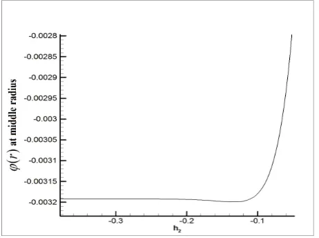
In order to show the influence of~i, i= 1,2 on the convergence ofmth-order approximations (in Eqs. 27),
u0(r) andw(r) are first plotted versus~i=,i= 1,2, re-spectively. The curvesu0(r) versus~iandw(r) against
~2 contain a horizontal line segment over the valid
re-gions. Liao called such kind of curve the~-curve [14], which clearly indicates the valid region of a solution series. In general, by means of ~-curves, it is straight forward to find the corresponding valid region of~. By choosing a value of ~ in the valid region, it can be ensured that the corresponding solution series is vergent to exact solution. In this way, one can con-trol and adjust the convergence region and rate of so-lution series. The ~-curve of u0(r) and φ(r) at the
mid-radius of rotating disk for 10th-order approxima-tion of them are shown in Fig. 1 and Fig. 2, respec-tively. From these figures, it is easy to discover that the valid region of ~1 for the given rotating disk is
−0.45 ≤~1 ≤ −0.2 and by attention to Fig. 2, valid
region of~2 is−0.4≤~2 ≤ −0.2. So, in this research,
the value of~1and~2are respectively selected -0.3 and
-0.27.
Fig. 1. ~1-curve of 10th-order approximation ofu0(r)
at middle radius of model D obtained by HAM.
Fig. 2. ~2-curve of 10th-order approximation of φ(r)
at middle radius of model D obtained by HAM.
3.2. Adomian’s Decomposition Method (ADM)
ADM approaches any equation, linear or nonlinear in a straight forward manner without any need to restric-tive assumptions such as discretization or perturbation [13]. Because of saving space, the background of ADM is not presented herein. In order to acquaint ADM, the audiences are referred to Author’s paper [9] and [13,24].
the linear operators Li, i = 1,2,3 corresponding to
u0(r), φ(r), w(r) can be respectively considered as:
L1[u0(r)] =
d2u 0(r)
dr2
L2[φ(r)] =
d2φ(r)
dr2 (29)
L3[w(r)] =
dw(r)
dr
The initial approximations presented in Eqs. (21) are also considered in ADM.
Considering Eqs. (19) and ADM algorithm, one can suggest the nonlinear operators Ni, i = 1,2,3 corre-sponding withu0(r), φ(r), w(r) respectively, as
N1[u0(r)] =
1
rEh d dr(rEh)
du0 dr + 1 rEh ( ν d
dr(Eh)− Eh
r
)
u0−
(1 +ν)
Eh d
dr(EhαT)
+(1−ν
2)ρrw2
E (30a)
N2[ϕ(r)] =
1
rh3E (
h3rdE dr +Eh
3+ 3h2dh
drEr
)
dφ dr
− 1
r2h3E (
−h3rνdE dr −3h
2dh
drErν+Eh
3 ) φ + 12 rEh3 (∫
rqzdr−c1 )
(1−ν2) (30b)
N3[φ(r)] =φ+
2
rEKh(1 +ν)
(∫
rqzdr
)
− 2c1
rEKh(1 +ν) (30c)
Now, Adomian’s polynomials Yi,m(m ≥0), i = 1,2,3 foru0(r), φ(r) andw(r) can be respectively determined
as the following equations:
Y1,m(u0,m) = 1
rEh d dr(rEh)
du0,m
dr
+ 1
rEh
(
ν d
dr(Eh)− Eh
r
)
u0,m
+ζm+1 [
−(1 +ν)
Eh d
dr(EhαT) +
(1−ν2)ρrw2
E
]
(31a)
Y2,m(φm) = 1
rh3E (
h3rdE dr +Eh
3+ 3h2dh
drEr
)
dφm
dr
− 1
r2h3E (
−h3rνdE dr −3h
2dh
drErν+Eh
3 )
φm
+ζm+1 12 (∫
rqzdr−c1 )
(1−ν2)
rEh3
(31b)
Y3,m(wm) =ϕm+ζm+1 [
2
rEKh(1 +ν)
(∫
rqzdr
)
− 2c1
rEKh(1 +ν)
]
(31c)
In ADM, the higher terms ofu0(r) are determined by
u0,m(r) =−L−1(N u0,m−1),m ≥1. This manner can
be followed to obtain the higher terms ofφ(r) andw(r). Hence, one has:
u0,m(r) =− ∫ ∫
Y1,m−1(u0,m−1)drdr+A1,m+B1,mr (32a)
φm(r) =−
∫ ∫
Y2,m−1(φm−1)drdr+A2,m+B2,mr (32b)
wm(r) =−
∫
Y3,m−1(φm−1)dr+A3,m (32c)
where A1,m, A2,m, A3,m and B2,m are integral con-stants which are determined by boundary conditions of Eq. (25). It is worth mentioning that c1 can also
be determined by boundary condition of Qr at outer radius of the disk.
By considering the disk model D (see Table 1), un-known functionsu0,m, φmandwmcan be obtained by substituting Eqs. (31) into Eqs. (32). Therefore, the
mth-order approximations ofu0, φ and w can be
ex-pressed, receptively, as the Eqs. (27).
Herein, Eqs. (27) are the solution expressions. By im-posing the boundary conditions (28) and using Eqs. (27) tou0, φandw(r) and Eqs. (14a), (14c) and (14d)
forNr, Qr and Mr, respectively, one can easily deter-mine the coefficientsA1,0, A2,0, A3,0, B1,0, B2,0 andc1.
3.3. Runge-Kutta’s Method (RK)
To calculate Eqs. (19) by well-known Runge-Kutta’s (RK) method, Eq. (19a), (19b) and (19c) must be solved in turn. In order to have numerical solution, the value of c1 of clamped-free boundary conditions
must be firstly obtained by the following equation:
c1= ∫
rqz(r)dr at r=b (33)
For numerical solution, Eqs. (19a) and (19b) have to be rewritten in the form of:
d2ψ dr2 =f
(
r, ψ,dψ dr
)
in whichψis a general unknown function. Here means
u0 orφwhich have the second order ordinary
differen-tial equations, i.e. Eqs. (19a) and (19b). In the RK method, the following equations are to be used [25]:
( dψ dr ) i+1 = ( dψ dr ) i +∆r
6 (K1+ 2k2+ 2k3+k4) (35a)
ψi+1=ψi+ ∆r
((
dψ dr
)
i +∆r
6 (k1+k2+k3) )
(35b)
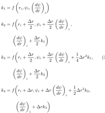
where ∆ris step length in the radial direction of the disk. Theki coefficients are calculated by
k1=f (
ri, ψi,
( dψ dr ) i )
k2=f (
ri+ ∆r
2 , ψi+ ∆r 2 ( dψ dr ) i , ( dψ dr ) i +∆r
2 k1 )
k3=f (
ri+ ∆r
2 , ψi+ ∆r 2 ( dψ dr ) i +1
4∆r 2
k1,
(
dψ dr
)
i +∆r
2 k2 )
k4=f (
ri+ ∆r, ψi+ ∆r
( dψ dr ) i +1
2∆r 2
k2,
(
dψ dr
)
i + ∆rk3
)
(36)
Eq. (19c) is a first-order differential equation which its solution by RK method needs to be proceeded by the following algorithm.
Eq. (19c) has to be firstly rewritten as the following equation:
dw
dr =g(r, w, φ) (37)
For the first order differential equation, following equa-tion is to be used [25]:
wi+1=wi+ 1
6(k1+ 2k2+ 2k3+k4) (38) where theki coefficients are calculated from
k1= ∆r(ri, wi, φi)
k2= ∆rg (
ri+ ∆r
2 , wi+ 1 2k1, φi
)
k3= ∆rg (
ri+ ∆r
2 , wi+ 1 2k2, φi
)
k4= ∆rg(ri+ ∆r, wi+k3, φi)
(39)
It is worth mentioning that execution of the numerical solution starts from the inner boundary with a trial
value of the first-order derivative of the unknown func-tions (u0 and φ). The procedure proceeds in an
it-erative and incremental manner. Here, the unknown functions can be determined by the boundary condi-tions on the outer radius of the disk. Mr and (for u0
andφ, respectively) must be equal to zero at outer ra-dius of the disk. In the next increment in the radial direction with the step length ∆r, the unknown func-tions and its first-order derivative at the new radius can be obtained using Eqs. (35). The unknown func-tionw, with initial valuew= 0 may be easily obtained by Eq. (38).
3.4. Finite Element Method (FE)
A finite element analysis of rotating disk with non-uniform thickness and material properties is performed using the commercial available software [26]. The ele-ment SHELL181 was used to analyze the problem. It is worthy to be said that SHELL181 is suitable for an-alyzing thin to moderately-thick shell structures. It is a four-node element with six degrees of freedom at each node: translations in the x, y, and z directions, and rotations about the x, y, and z-axes. SHELL181 is well-suited for linear, large rotation and large strain nonlinear applications. The accuracy in modeling is governed by the Mindlin’s first-order shear deforma-tion theory [26].
It is noted that in the present study, the element SHELL181 was used in the elastic zone to analyze the bending of thin and moderately-thick rotating disks. Fig. 3 shows the modeled rotating disk and imposing associated loading and boundary conditions. As seen in Fig. 3, in order to decrease CPU-time, the one-fourth disk was modeled and then the associated boundary conditions were imposed as will be next explained.
Fig. 3. Finite element model, meshing and imposing boundary conditions (Real meshing is so much finer).
one-fourth-modeled rotating disk, the symmetric boundary condi-tions in two edges of the model at degree of zero and
π/2 radians were imposed. The inner radius of the disk was clamped by constraining all degree of freedoms, i.e. UX, UY, UZ, ROTX, ROTY and ROTZ. The outer ra-dius of the disk, which is free of any traction, was held unchanged. In order to achieve the adequate accuracy, the disk was discretized into 100 segments in radial di-rection. In each segment, the thickness and properties of disk were assumed constant and corresponding to their values at given radius defined by Eqs. (1) and (2).
4. Results and Discussion
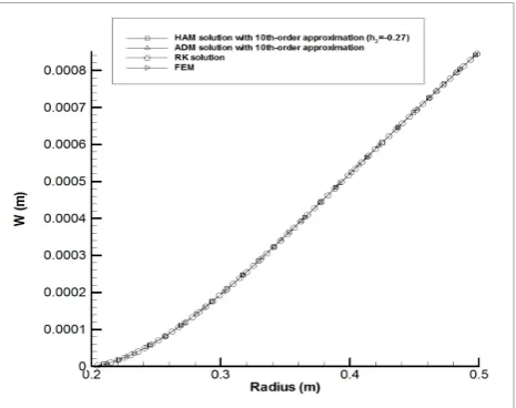
In this section, results from HAM and ADM are pre-sented and compared with those obtained by Runge-Kutta’s and finite element solution. Fig. 4 to Fig. 6 show the distribution of functionsu0(r),φ(r) andw(r)
against disk radius resulted by HAM, ADM, RK, and FEM for disk model D respectively.
Fig. 4. The distribution of functionu0(r) obtained by
HAM, ADM, RK and FEM for model D.
Fig. 5. The distribution of functionφ(r) obtained by HAM, ADM, RK and FEM for model D.
Fig. 6. The distribution of functionw(r) obtained by HAM, ADM, RK and FEM for model D.
Fig. 7. Comparison of calculated stresses by HAM, ADM, RK and FEM of model D atz=−h(r)/2.
Fig. 8. The distribution ofu0(r) versus the radius of
Fig. 9. The distribution of w(r) versus the radius of the disk with respect to the angular velocity.
Fig. 10. The distribution of u0(r) versus the radius
of the disk with respect to the temperature gradient.
Fig. 11. The distribution ofw(r) versus the radius of the disk with respect to the temperature gradient.
Fig. 12. The distribution of u0(r) versus the radius
of the disk with respect to the lateral pressure.
Fig. 13. The distribution ofw(r) versus the radius of the disk with respect to the lateral pressure.
Fig. 14. The distribution of u0(r) versus the radius
Fig. 15. The distribution ofw(r) versus the radius of the disk with respect to the grading index.
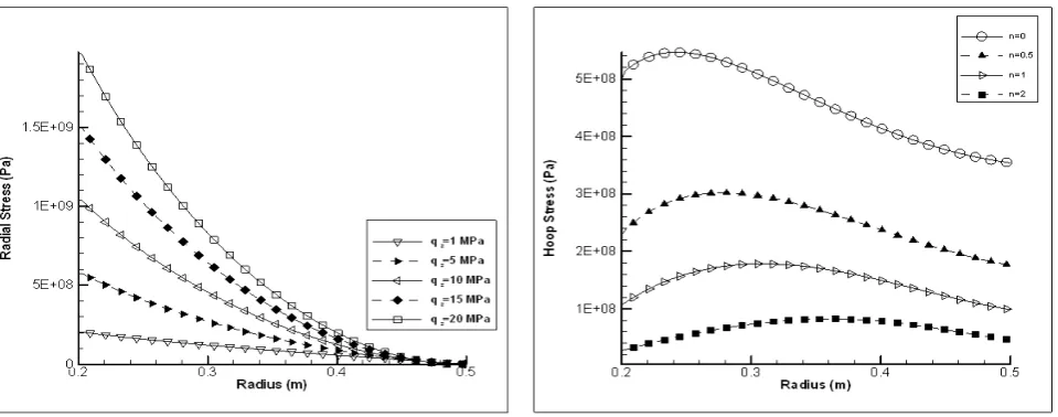
Fig. 16. The radial stress versus the radius of the disk with respect to the lateral pressure.
Fig. 17. The hoop stress versus the radius of the disk with respect to the lateral pressure.
Fig. 18. The radial stress versus the radius of the disk with respect to the grading index.
Fig. 19. The hoop stress versus the radius of the disk with respect to the grading index.
Fig. 21. The hoop stress versus the radius of the disk with respect to the angular velocity.
By using the solution ofu0(r), φ(r) and and
apply-ing Eqs. (5), one can easily obtain the distributions of components of stress. Fig. 7 presents the radial and hoop stresses of disk model D atz =−h(r)/2, calcu-lated by HAM, ADM, RK and FE methods. Fig. 4 to Fig. 7 obviously display that the results of four meth-ods are in excellent agreements. Therefore, it induces that practiced methods have excellent ability of solving the moderately thick functionally graded thermoelastic rotating disks subjected to bending loading based on the Mindlin’s theory.
In model D at z = −h(r)/2, the maximum stress component is the radial stress occurring at inner ra-dius of the disk. The radial stress continuously reduces from the maximum point at inner radius to minimum position at outer radius. By considering Fig. 7, it is obvious that the hoop stress has its minimum value at inner radius, while; its maximum value occurs at outer radius of the disk. The hoop stress increases from inner radius up to a position within the disk, then decreases from that position up to another position within the disk, and then again increases from the latter position up to its maximum value at outer radius. It is worth-while that the variations of hoop stress of model D against those of radial stress are trivial. In addition, it is necessary to notice that if there is no thermal loading, the angular velocity leads to positive radial and hoop stresses throughout the disk. Whereas, the thermal loading alone causes the negative hoop stress throughout the disk. As seen in Fig. 7, the circum-ferential stress is negative throughout the disk due to imposing both the angular velocity and thermal load-ing, simultaneously. It means that in the special model of the disk and loading (model D), presented in Table (1), the influence of thermal loading is greater than that of angular velocity to distribute the hoop stress of the rotating disk.
As final words, it can be said that the
implemen-tation of the proposed methods demonstrates the ap-plicability of the HAM and ADM to provide accurate enough solution for a complicated case with no exact solution.
Fig. 8 and Fig. 9 show the variations of u0 and
w with the changes of the angular velocity w of the model D, respectively. Fig. 8 and Fig. 9 demonstrate that the radial displacement of the middle surface of the disk u0(r) increases with the increase in angular
velocity, whereas angular velocity plays no role in de-termination of deflectionw. This implies the fact that the differential equations ofu0(r) andw(r) are
uncou-pled due to linearity. In the other words, the unknown functions u0(r) and w(r) are coupled if the
govern-ing differential equations are non-linear. Fig. 10 and Fig. 11 show the influence of temperature on the ra-dial displacement, u0, and deflection, w, respectively.
As seen in Fig. 10, the increase in temperature gives rise to increase in radial displacement of mid-planeu0,
while the variations of temperature has no influence on the deflection. This fact can be easily derived through differential equations (15b) and (15c). The terms αT
doesn’t exist in the equations related to w and ϕ. In the view of physical interpretation, when there are no temperature gradients in thickness direction, it is not expected any deflection. Fig. 12 and Fig. 13 display the variations of radial displacementu0and deflection
w against lateral pressureqz. As revealed in Fig. 12, the lateral loading qz plays no role in radial displace-ment of the middle surface of the disk. This is fully comprehended due to the concepts of Mindlin’s theory of plates. It is that the middle surface of the plate has no stretch due to bending loading. As it can be seen in Fig. 13, the increase in lateral pressure qz causes increase in deflectionw. Fig. 14 and Fig. 15 show the role of grading index on the radial displacement, u0,
and the deflection,w. As seen, the increase in grading index gives rise to decrease in bothu0 andw. Fig. 16
and Fig. 17 display the influence of lateral pressureqz on the radial and circumferential stresses, respectively. As expected, the growth of lateral pressure leads to in-crease in both components of stress. Fig. 18 and Fig. 19 present the effect of grading index on the radial and circumferential stresses respectively. As it can be seen, the increase in grading index results in decrease in ra-dial and hoop stresses. It can be resulted from Fig. 14 and Fig. 15 related to the influence of grading index on u0 and w. It is obvious that the increase in both
u0 andw are generally resulted in growth of both
ra-dial and hoop stresses. Fig. 20 and Fig. 21 show the role of angular velocity on the radial and hoop stresses respectively. As it can be expected, the increase in an-gular velocity leads to increase in both radial and hoop stresses.
radial and hoop stresses, the temperature and its ef-fects are vanished. In the other words, the temperature is only considered to derive Fig. 1 to Fig. 7 and Fig. 10 and Fig. 11.
5. Conclusions
In this paper, firstly, the governing differential equa-tions of FGM rotating disk with variable thickness sub-jected to thermo-elastic and bending loadings through Mindlin’s first order shear deformation theory were ex-tracted. Then, two methods, namely Liao’s homo-topy analysis method (HAM) and Adomian’s decom-position method (ADM) were applied to analyze the moderately-thick rotating disk. Such a study is unde-niably required to realize how to treat some compo-nents such as brake disk and clutch. Comparing the results obtained by two methods with those of Runge-Kutta’s and finite element methods (FEM), the cor-rectness and reliability of the proposed methods for analysis of rotating disk were proven. With the help of results obtained by four methods, the components of stress were easily obtained by using calculated u0(r),
φ(r) and w(r) in HAM, ADM, RK and FEM. The curves and its variations of radial and hoop stresses of rotating disk were surveyed. For further investigation, the effects of angular velocity, lateral pressure, tem-perature and grading index on the radial displacement of mid-plane of the disk, deflection and on the radial and hoop stresses were demonstrated and discussed in detail.
References
[1] M. Bayat, B.B. Sahari, M. Saleem, A. Ali, S.V. Wong, Bending analysis of a functionally graded rotating disk based on the first order shear defor-mation theory, Appl. Math. Model., 33 (2009) 4215-4230.
[2] A.N. Eraslan, Y. Orcan, Elasticplastic deformation of a rotating solid disk of exponentially varying thickness. Mech. Mater., 34 (2002) 423-32.
[3] S.A.H. Kordkheili, R. Naghdabadi, Thermoelas-tic analysis of a functionally graded rotating disk, Compos. Struct., 79 (2006) 508-16.
[4] M. Bayat, M. Saleem, B.B. Sahari, A.M.S. Hamouda, E. Mahdi, Mechanical and thermal stresses in a functionally graded rotating disk with variable thickness due to radially symmetry loads, Int. J. Pres. Ves. Pip., 86 (2009) 357-372.
[5] M.H. Hojjati, S. Jafari, Variational iteration solu-tion of elastic non uniform thickness and density rotating disks, Far. East. J. Appl. Math., 29 (2007) 185-200.
[6] M.H. Hojjati, S. Jafari, Semi-exact solution of elastic non-uniform thickness and density rotating disks by homotopy perturbation and Adomian’s de-composition methods. Part I: Elastic solution, Int. J. Pres. Ves. Pip., 85 (2008) 871-879.
[7] M.H. Hojjati, S. Jafari, Semi-exact solution of non-uniform thickness and density rotating disks. Part II: Elastic strain hardening solution, Int. J. Pres. Ves. Pip., 86 (2009) 307-18.
[8] M.H. Hojjati, A. Hassani, Theoretical and numeri-cal analyses of rotating discs of nun-uniform thick-ness and density, Int. J. Pres. Ves. Pip., 25 (2008) 695-700.
[9] A. Hassani, M.H. Hojjati, G. Farrahi, R.A. Alashti, Semi-exact elastic solutions for thermo-mechanical analysis of functionally graded rotating disks, Com-pos. Struct., 93 (2011) 3239-3251.
[10] A. Hassani, M.H. Hojjati, G. Farrahi, R.A. Alashti, Semi-exact solution for thermo-mechanical analysis of functionally graded elastic-strain hard-ening rotating disks, Commun. Nonlinear. Sci. Num. Simulat., 17 (2012) 3747-3762.
[11] A. Hassani, M.H. Hojjati, E. Mahdavi, R.A. Alashti, G. Farrahi, Thermo-mechanical analysis of rotating disks with non-uniform thickness and ma-terial properties, Int. J. Pres. Ves. Pip., 98 (2012) 95-101.
[12] A. Hassani, M.H. Hojjati, A.R. Fathi, In-Plane free vibrations of annular elliptic and circular elas-tic plates of non-uniform thickness under classi-cal boundary conditions, Int. Rev. Mech. Eng., 4 (2010) 112-119.
[13] G. Adomian, Solving frontier problems of physics: the decomposition method. Boston: Kluwer Aca-demic; 1994.
[14] S.J. Liao, Beyond perturbation: introduction to the homotopy analysis method. Boca Raton: Chap-man and Hall/CRC Press; 2003.
[15] S.A. Hosseini Kordkheili, M. Livani, Thermoe-lastic creep analysis of a functionally graded var-ious thickness rotating disk with temperature-dependent material properties, Int. J. Pres. Ves. Pip., (2013) 63-74.
[17] D. Ting, D. Hong-Liang, Thermo-elastic analy-sis of a functionally graded rotating hollow circu-lar disk with variable thickness and angucircu-lar speed, Appl. Math. Model., 40 (2016) 7689-7707.
[18] Hong-Liang Dai, Zhen-Qiu Zheng, Ting Dai, In-vestigation on a rotating FGPM circular disk under a coupled hygrothermal field, Appl. Math. Model., 46 (2017) 28-47.
[19] D. Ting, D. Hong-Liang, An analysis of a rotating (FGMEE) circular disk with variable thickness un-der thermal environment, Appl. Math. Model., 45 (2017) 900-924.
[20] R. Szilard, Theories and applications of plate anal-ysis: Classical, Numerical and Engineering Meth-ods, John Wiley & Sons, Inc; 2004.
[21] S. Chakraverty, Vibration of plates, New York: CRC Press; Taylor & Francis group; 2009.
[22] S.S. Rao, Vibration of continuous systems, John Wiley & Sons, Inc; 2007.
[23] J.N. Reddy, C.M. Wang, S. Kitipornchai, Axisym-metric bending of functionally graded circular and annular plate, Eur. J. Mech. A/Solids 18 (1999) 185-199.
[24] A.M. Wazwaz, Partial differential equations and solitary waves theory, Higher education Press, 2009.