tobac 1.2: towards a flexible framework for tracking and analysis of clouds in diverse datasets

https://doi.org/10.5194/gmd-12-4551-2019 © Author(s) 2019. This work is distributed under the Creative Commons Attribution 4.0 License.

tobac 1.2: towards a flexible framework for tracking

and analysis of clouds in diverse datasets

Max Heikenfeld1, Peter J. Marinescu2, Matthew Christensen1, Duncan Watson-Parris1, Fabian Senf3, Susan C. van den Heever2, and Philip Stier1

1_{Atmospheric, Oceanic & Planetary Physics, Department of Physics, University of Oxford, Oxford, UK} 2_{Department of Atmospheric Sciences, Colorado State University, Fort Collins, USA}

3_{Leibniz Institute for Tropospheric Research, Leipzig, Germany} Correspondence:Philip Stier ([email protected]) Received: 14 April 2019 – Discussion started: 24 May 2019

Revised: 14 September 2019 – Accepted: 19 September 2019 – Published: 30 October 2019

Abstract. We introduce tobac (Tracking and Object-Based Analysis of Clouds), a newly developed framework for track-ing and analystrack-ing individual clouds in different types of datasets, such as cloud-resolving model simulations and geo-stationary satellite retrievals. The software has been designed to be used flexibly with any two- or three-dimensional time-varying input. The application of high-level data formats, such asIriscubes orxarrayarrays, for input and output allows for convenient use of metadata in the tracking analysis and visualisation. Comprehensive analysis routines are pro-vided to derive properties like cloud lifetimes or statistics of cloud properties along with tools to visualise the results in a convenient way. The application of tobac is presented in two examples. We first track and analyse scattered deep convec-tive cells based on maximum vertical velocity and the three-dimensional condensate mixing ratio field in cloud-resolving model simulations. We also investigate the performance of the tracking algorithm for different choices of time resolu-tion of the model output. In the second applicaresolu-tion, we show how the framework can be used to effectively combine in-formation from two different types of datasets by simultane-ously tracking convective clouds in model simulations and in geostationary satellite images based on outgoing longwave radiation. The tobac framework provides a flexible new way to include the evolution of the characteristics of individual clouds in a range of important analyses like model intercom-parison studies or model assessment based on observational data.

1 Introduction

approaches, which are often based on bulk statistical prop-erties over larger regions in space and time, such as entire modelling or observational domains. Model intercompari-son studies with cloud-resolving model (CRM) simulations have mostly relied on the comparison of domain and time-averaged quantities or similar statistics (Varble et al., 2011; Varble et al., 2014a, b; Fan et al., 2017). This generally lim-its the investigation of differences between the models on the scale of individual convective cells or analyses that take the temporal evolution of individual clouds into account.

Any analysis focused on the properties of individual clouds in larger databases containing numerous cloud ele-ments and aimed at including the time evolution over their development cycle requires some form of cloud tracking technique. A large body of work exists on tracking individual clouds in different types of data, ranging from ground-based radar and geostationary satellite retrievals to model simula-tions at a range of different resolusimula-tions. We now present a short but certainly not exhaustive overview of existing ap-proaches. This will be used to show the capabilities of the existing software and to discuss the drawbacks and limita-tions which motivated the development of the more flexible software framework tobac (Tracking and Object-Based Anal-ysis of Clouds) presented here.

Tracking individual convective clouds in radar data has been performed for decades (Crane, 1979; Rosenfeld, 1987). These efforts were often motivated by their use in nowcast-ing of severe weather warnnowcast-ings, e.g. for floodnowcast-ing due to con-vective precipitation, damage from hail or impacts of high wind speeds such as tornadoes (Dixon and Wiener, 1993; Lakshmanan and Smith, 2009). The satellite-based track-ing of convective clouds has been performed both with a similar focus on nowcasting convection and for long-term analysis in climate research (Menzel, 2001; Sieglaff et al., 2012). Special tracking algorithms that combine information from different wavelength bands of imagers on geostationary satellites, such as Cb-TRAM (Zinner et al., 2008, 2013) and RTD (Autonès and Moisselin, 2013), have been developed as tools to identify and track deep convective clouds throughout their development cycle, including the initial stage of rising cumulus towers. However, both products have been devel-oped for a specific application that strongly limits a more general adaption of the software by the user. Several other studies have used geostationary satellite data to investigate the growing phase and glaciation of deep convective clouds (Mecikalski and Bedka, 2006; Mecikalski et al., 2011; Senf et al., 2015; Senf and Deneke, 2017). Other applications have specifically focused on the analysis of long-lived MCSs over different regions of the globe (Machado et al., 1998; Feng et al., 2012, 2018; Hagos et al., 2013). The identification of individual cloud objects in satellite data is one aspect of cloud tracking and has been used to investigate the spatial scaling of clouds on a global scale (Wilcox and Ramanathan, 2001; Wood and Field, 2011), including studies on the rep-resentation of these distributions in global atmospheric

mod-els (Wilcox, 2003; O’Brien et al., 2013). The use of satellite data from active sensors (Nesbitt et al., 2000; Bacmeister and Stephens, 2011; Riley et al., 2011; Igel et al., 2014; Guil-laume et al., 2018) allows for the inclusion of information about the vertical extent of identified cloud objects, which provides an improved classification of cloud types and un-derstanding of important physical processes.

Tracking individual cloud objects in high-resolution CRM simulations and large-eddy simulation (LES) models has been developed alongside the evolution of these simulations in recent decades. Earlier studies on tracking shallow convec-tion in high-resoluconvec-tion model simulaconvec-tions (Zhao and Austin, 2005a, b; Heus et al., 2009) strongly relied on manual de-tection techniques. Subsequently, Dawe and Austin (2012) and Heus and Seifert (2013) presented automated methods of tracking shallow convection that rely on a continuous release of a decaying tracer from the model as described in Couvreux et al. (2010). However, the functionality of the tracer re-lease and advection must be specifically implemented in each model and restricts the use of this technique to the output of high-resolution models. Cloud tracking algorithms applied online during the actual model simulations (Plant, 2009) have the advantage of direct access to the relevant model fields at the model time step and thus the highest possible time reso-lution. However, these online algorithms must also be imple-mented separately in a specific model.

domains or simulations for longer time periods. Providing adequate ways of performing tracking and object-based anal-yses for different types of clouds, including deep convection, in these kinds of simulations provides a key pathway to better understanding the underlying physical processes.

This overview clearly shows the wide range of exten-sive efforts that went into the development of elaborate soft-ware and analysis tools to track clouds in different types of datasets. The application of cloud identification and tracking and related techniques has substantially increased our under-standing of cloud size distributions, the time evolution of dif-ferent types of clouds, and the underlying physical processes governing cloud formation, development, and propagation. However, the overview also highlights the problem of lim-ited compatibility between the different existing approaches and implementations, especially regarding the intended use of tracking clouds based on different data sources using the same algorithms and analysis tools.

To address some of these limitations of existing ap-proaches and provide a more functional tool with increased flexibility for different applications, we have developed tobac as a new flexible software tool for the identification, tracking and analysis of clouds. This approach certainly does not in-tend to replace the existing tools in their specific applications, but it rather aims to provide a flexible framework that can be used for a wide range of different datasets and also allows for the future integration of some of the existing approaches discussed here.

We have designed tobac in a modular way that includes the following basic steps, which are described in detail in Sect. 2.1–2.5:

1. data input and output; 2. feature detection;

3. segmentation of cloud areas and volumes; 4. trajectory linking; and

5. object-based analysis and visualisation.

The tobac framework allows for a convenient application to output from a wide range of model simulations and obser-vational products, as long as it is provided with sufficient temporal and spatial resolution and contains output variables that can be used to identify individual clouds. Therefore, the software package can be used for a range of important appli-cations like model intercomparison studies, which generally rely on simpler analysis methods that do not capture the evo-lution of individual clouds. These capabilities also allow for comparative studies between model simulations and obser-vational datasets, e.g. from satellite retrievals, using the same underlying statistical methods. Due to the modular structure, tobac is set up for the integration of existing or newly devel-oped algorithms for the different steps in the analysis chain. The implementation in Python provides tobac with access

to numerous more specialised existing software libraries for different aspects of the software, such as data input–output, memory usage and the existing functionality from the field of image processing. We also show how we can leverage an existing Python library from an entirely different field of the physical sciences to perform integral parts of the linking step in our application. Furthermore, the choice of Python for to-bac makes the package more easily accessible to users as it allows for easier integration into existing analysis workflows and also stimulates the integration of additional components in the modular workflow of the package.

To show the advantages of tobac in practical applications, we present two different examples of using the framework in tracking and analysing deep convective clouds. In the first application, the detection of features is performed on the column-maximum vertical velocity at each output time in-terval from a CRM simulation. A three-dimensional water-shedding algorithm is applied to the updraft field and to the total condensed water content field (mass mixing ratio of all hydrometeors) at each step in time to infer both the volume of the individual updrafts and the clouds associated with the tracked updrafts. These features are then filtered and linked into consistent trajectories. We use the tracking results to as-sess the distribution of cloud lifetimes and the requirements for the model output temporal resolution. In the second ap-plication, we perform a simultaneous analysis for model and satellite data. Similar vertically resolved data as used in the other example are usually not available from satellite im-agers. The information in most satellite retrievals of cloud properties is limited to two dimensions. With a multi-spectral selection of channels from the satellite instrument, cloud-top height and radiative properties can be retrieved (McGarragh et al., 2018). An analysis of model-simulated and satellite-retrieved fields of outgoing longwave radiation (OLR) is pre-sented to demonstrate the flexibility of the tobac approach. By making use of the framework consistently across differ-ent datasets like this, we can compare the tracked clouds in both data sources by examining the statistical properties of the resulting population of convective clouds, thereby facili-tating model–observation comparisons.

2 Software description

2.1 Data input and output

The input data for the framework are provided in a high-level format of either Iris cubes (Met Office, 2018) or xarraydata arrays (Hoyer and Hamman, 2017), which in-clude detailed metadata for each data variable, such as units and coordinates. The algorithm can thus automatically use these metadata, and the tracking setup can be controlled in-dependently of the temporal resolution, spatial resolution or dimensions of the input data. Tracking parameters represent-ing physical properties like distances or time periods can be set in physical units and are automatically converted to pixel-based values needed for the underlying calculations. Scien-tific data are provided in a vast variety of different file for-mats and data structures. Implementing a way of loading the data into the right format for an application often proves to be a significant limitation to the use of new datasets and gen-erally consumes an unjustifiable amount of time and effort, apart from providing an important source of implementation errors. The Python library Community Intercomparison Suite (CIS) (Watson-Parris et al., 2016) overcomes this challenge and provides a convenient way to automatically load a vast array of observational datasets intoIris-compatible objects for direct use in tobac.

Both Iris and xarray make use of so-called “lazy loading” based on thedaskpackage (Rocklin, 2015; Dask Development Team, 2016) for efficient memory usage. The initial loading of data from a file only creates a placeholder. Then, individual operations on the data are combined and evaluated once the final result is to be saved, printed or plot-ted. Only at this stage are data actually loaded from a disk into the physical memory of the computing machine and in-dividual calculations performed. Based on these capabilities, the entire tobac framework is written with a focus on limit-ing instantaneous memory usage by splittlimit-ing up calculations into chunks, e.g. along the time dimension. Hence, even large datasets with individual fields much larger than the memory available on the computing system can be conveniently pro-cessed without special adaptation by the user.

The output of the tracking analysis is given in commonly used high-level Python data format aspandasdata frames (McKinney, 2010) for a table containing the tracked cell cen-tres and trajectories and asIriscubes orxarraydata ar-rays for the masks of cloud volumes or areas. This output is automatically amended with the same metadata as the input data like coordinates (e.g. time, longitude, latitude), along with additional information from the tracking process, e.g. a time coordinate relative to the initiation of an individual con-vective cell. This allows for the convenient and direct use of the output for visualisation and further analyses. The inter-mediate results of each individual analysis step can be con-veniently saved and examined in the form ofpandasdata frames orIriscubes.

2.2 Feature detection

The feature detection can work with any two-dimensional field either present or derived from the input data. In the first example, we use maxima in the maximum vertical velocity in each column of the three-dimensional high-resolution model output to identify individual updrafts (see Sect. 3). In the sec-ond example, minima in outgoing longwave radiation from satellite retrievals and model output are used in the feature detection (see Sect. 4).

To identify the features, contiguous regions above or below a threshold are determined and labelled individu-ally. Smoothing the input data, e.g. with a Gaussian fil-ter, can make this step more reliable. The detection of re-gions above a specific threshold can lead to large intercon-nected regions combining several features linked by narrow ridges. To prevent this and identify these interconnected fea-tures separately, the tobac feature detection allows for the use of “erosion” techniques based on the implementation in skimage.morphology.binary_erosion. These techniques shrink the identified regions from the edges by a specific length or number of pixels, thus removing the connecting ridges between interconnected features. This has been shown to lead to more robust detection of individual features, as described in detail in Senf et al. (2018).

To describe the specific location of the feature at a specific point in time, we have investigated the use of different spa-tial properties describing the identified region. The geometric centre can be strongly affected by changes in the shape of the boundary, which is determined based on the selected thresh-old value. Instead, we have found that a weighted mean

xmean=

X

i

wixi, (1)

with weightswigiven by the difference between the values of the chosen field at the individual pointsViand the threshold valueVfeature,

wi=_PVi−Vfeature iVi−Vfeature

, (2)

has proven to perform best in determining a robust feature position. We can interpret this position as the centre of mass of the component of the field exceeding the chosen threshold value.

Figure 1.Schematic overview of the general workflow of the tobac tracking analysis framework and of the two examples presented in this paper.

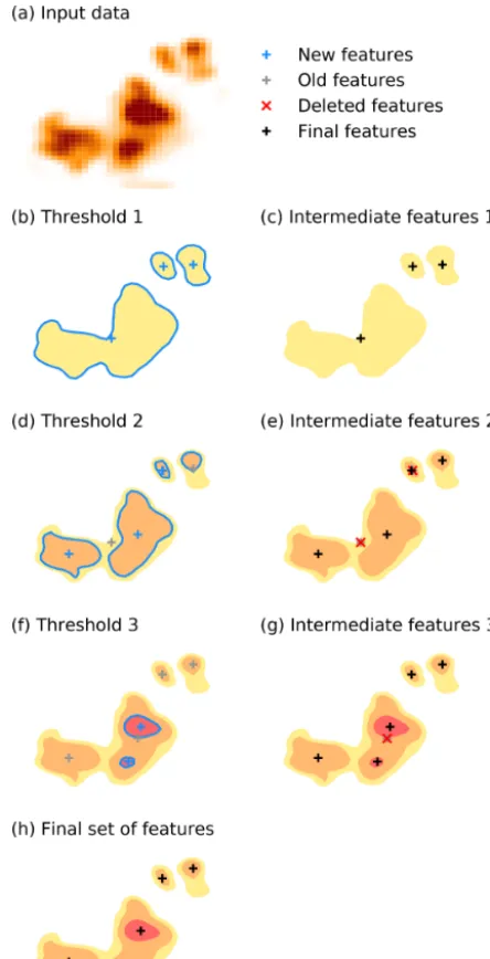
(Fig. 2). These threshold values have to be chosen specifi-cally for each application of tobac. The choice can be based on a detailed analysis of the data used for tracking to deter-mine where the features separate from the background, e.g. based on histograms as shown in Sect. 4, or using empiri-cal values from previous studies of the specific phenomena. The feature identification starts with labelling the regions for the least restrictive threshold. For each threshold value, fea-tures are identified in the same way (Fig. 2b, d, f) and replace existing features that were found based on a less restrictive threshold value in the surrounding region (Fig. 2e, g).

This combination of different thresholds allows tobac to detect lower-intensity features representing weaker convec-tive clouds or clouds in their initial or decay stage but identify localised features with stronger updrafts or colder cloud tops within the weaker-threshold areas. In the first example ap-plication (Sect. 3), consecutive maximum updraft threshold values of 3, 5 and 10 m s−1were used, while tracking based on OLR in the second example (Sect. 4) was performed with consecutively smaller threshold values (250, 225, 200, 175 and 150 W m−2). While using multiple thresholds is usually beneficial, feature detection using a single threshold value is possible in tobac by only supplying a single threshold value and can be appropriate in certain applications.

An iterative set of threshold values was used in other re-cent approaches to cloud detection (Liang et al., 2017; Fu et al., 2019) but with a specific focus on application to cer-tain types of satellite images. Multiple-threshold methods are also applied in other fields of science facing similar chal-lenges in feature detection such as astronomy (Zheng et al., 2015).

2.3 Segmentation

Once features and feature centres are identified, segmen-tation techniques are used to associate areas or volumes with each identified feature. In the current version of the tobac framework, we have implemented segmentation us-ing watersheddus-ing techniques from the field of image pro-cessing (skimage.morphology.watershedfrom the scikit-imagelibrary; Soille and Ansoult, 1990; van der Walt et al., 2014) with a fixed threshold valueVsegmentation. This value has to be set specifically for every type of in-put data and application, as explained in more detail for the two example applications in Sects. 3 and 4. Watershedding segmentation treats the input field as a topographic map and separates the input into individual regions similar to individ-ual watersheds or catchment basins along a dividing ridge in a geological context (Meyer, 1994). These techniques are widely used in several existing cloud tracking and analy-sis algorithms described in Sect. 1, such as Heiblum et al. (2016a), Fiolleau and Roca (2013), and Senf et al. (2018).

Figure 2.Schematic illustration of the multi-threshold feature de-tection approach using three different threshold values.

between the two regions. This procedure creates a mask of the same shape as the input data, with zeros at all grid points in which there is no cloud or updraft and the integer number of the associated feature at all grid points belonging to that specific cloud or updraft. This mask can be conveniently and efficiently used to select the volume of each cloud object at a specific time step for further analysis or visualisation.

The structure of tobac allows for the future implementa-tion of other algorithms for the segmentaimplementa-tion step, e.g. re-placing the watershedding approach by random walk tech-niques (Grady, 2006; Wang et al., 2019) or other image pro-cessing tools. Similarities between the feature detection and segmentation steps mean that these steps could be combined in some implementations in future versions of tobac, e.g. for

Figure 3.Schematic illustration of the trajectory linking with the predicted motion of the feature based on previous time steps and a search range around the predicted position.

applications based on a single input dataset (OLR), as used in Sect. 4. However, treating the two analysis steps separately allows for the combination of different datasets (vertical ve-locity and condensed water content), as shown in Sect. 3. 2.4 Trajectory linking

The individual features and associated areas and volumes identified in each time step have to be linked into cloud tra-jectories to analyse the time evolution of cloud properties for a better understanding of the underlying physical processes. For this step, we have implemented a linking method that makes use oftrackpy(Allan et al., 2016), a Python library originally developed for tracking particles and cells in micro-scopic images. The linking determines which of the features detected in a specific time step (see Sect. 2.2) is identical to an existing feature in the previous time step and is illustrated in Fig. 3. For each existing feature, the movement within a time step is predicted based on the velocities in a number of previous time steps. The algorithm then breaks the search process down to candidate features by restricting the search to a circular search region centred around the predicted posi-tion of the feature in the next time step. For newly initialised trajectories, for which no velocity from previous time steps is available, the algorithm resorts to the average velocity of the nearest tracked objects. The parametervmaxrestricts how much the future position of a feature is allowed to deviate from a linear extrapolation of the trajectory over time. It thus has the units of a velocity and describes the dependency of the circular search ranged on the output time step1tin the data used for the tracking:

d=vmax1t. (3)

radius of the search rangedmin(2 km, equivalent to 4 times the grid spacing in Sect. 3) that specifies a lower limit for the size of the search region. Both these parameters are given as physical quantities and then converted into pixel-based val-ues used intrackpy. This allows for cloud tracking that is controlled by physically based parameters that are indepen-dent of the temporal and spatial resolution of the input data. We make use of this for cloud tracking with different model output frequencies for the same simulations in the example application in Sect. 3.

Features can be allowed to be missed for a certain number of time steps (memory) and still get linked into a trajectory. However, this option should be used with caution, as it can lead to erroneous trajectory linking, especially for data with low time resolution. For example, convective clouds can pro-duce outflow boundaries that initiate new convective clouds nearby, and the newly formed clouds are more likely to be linked to the original clouds with this option.

The feature detection step can often omit the initial or fi-nal stages of the evolution of a cloud due to the choice of specific thresholds. Thus, trajectories can also be extrapo-lated to additional output time steps at the start and at the end of the tracked path. This allows for the inclusion of both the initiation of the cell and the decaying later stages in the analysis of the cloud life cycle. Furthermore, a threshold for the minimum lifetime of the tracked objects can be used to exclude the analysis of clouds that have only been tracked for a very short period and are likely to be spurious features. Such tracked objects can contaminate analyses focusing on the cloud lifetime and associated quantities.

The trajectories are recorded in a pandas data frame. This enables the filtering of the resulting trajectories, e.g. to reject trajectories that are only partially captured at the boundaries of the input field both in space and time.

The current implementation of the linking step does not include an explicit treatment of the splitting and merging of clouds, as implemented in several of the cloud tracking algo-rithms reviewed earlier (Dawe and Austin, 2012; Heus and Seifert, 2013; Heiblum et al., 2016a). Instead, the current ver-sion of tobac will create a continuous track with only one of the two separate cloud objects that combine in a merger or evolve from the splitting of a tracked object, mostly based on which of these has the more similar direction of travel to the joint object. However, we have structured the implemen-tation of tobac in a way that allows for the future addition of more complex tracking methods that can record a more complex network of relationships between cloud objects at different points in time.

2.5 Object-based analysis and visualisation

To make use of the results of the previous steps, we pro-vide detailed tools to analyse and visualise the tracked ob-jects. We provide a set of routines that enable the perfor-mance of analyses and the derivation of statistics for

indi-vidual clouds, such as the time series of integrated properties and vertical profiles. We also provide routines to calculate summary statistics of the entire population of tracked clouds in the cloud field like histograms of cloud areas and volumes or cloud mass and a detailed cell lifetime analysis (see Figs. 6 and 10).

These analysis routines are all built in a modular manner. Thus, users can reuse the most basic methods for interacting with the data structure of the package in their own analy-sis procedures in Python. This includes functions performing simple tasks like looping over all identified objects or cloud trajectories and masking arrays for the analysis of individual cloud objects. Plotting routines include both visualisations of the entire cloud field and detailed visualisations for individ-ual convective cells and their properties.

2.6 Advantages of the implementation in Python While the majority of the existing tracking approaches re-viewed in Sect. 1 are implemented either in Fortran, C and C++, or in proprietary programming languages like MAT-LAB, we have chosen to use Python for our tracking frame-work for several practical reasons. Python has become the go-to standard for data analysis in many fields of scien-tific research, including the atmospheric sciences in recent years (Lin, 2012; Perkel, 2015). This makes it possible to develop software that is accessible and modular, which al-lows for the successful addition of user-contributed algo-rithms or the adoption or application of the workflow for cases beyond those presented here. The use of libraries in the scientific Python ecosystem includingNumPy,SciPy, andmatplotlib(Hunter, 2007; van der Walt et al., 2011), along with a large stack of existing and optimised libraries providing image processing features (van der Walt et al., 2014), means that the package is based on actively developed open-source projects. This ensures an accurate, effective and tested implementation of the individual calculations as well as the continuous integration of new developments and im-provements. Most of these Python libraries use Fortran or C for the actual underlying calculations, which means that many of the individual operations within tobac make use of the increased computational speed of these languages. The use of Python also means that even users without extensive programming experience will be able to easily adapt existing procedures into the workflow or contribute additional algo-rithms to the modular structure of the tobac tracking frame-work.

The implementation in Python also enables the use of Jupyter notebooks (Perez and Granger, 2007; Kluyver et al., 2016) as an innovative way of developing, visualising and sharing scientific data analyses. We provide examples of the analyses presented here as Jupyter notebooks in the software package.

(Dawe and Austin, 2012; Heus and Seifert, 2013). The use of modern memory management techniques such as “lazy data loading” in the underlying Python libraries Iris(Met Of-fice, 2018) andxarray(Hoyer and Hamman, 2017), which both rely on dask data types (Rocklin, 2015), allows for clear and concise source code while sparing users the experi-ence of having to deal with most memory-related considera-tions themselves. Memory usage and algorithm run time for the two applications presented in this paper are included in the following sections.

3 Example A: tracking convective cells in

high-resolution model simulations based on updraft velocities and condensate mixing ratios

In the first example, we apply the tracking framework to CRM simulations of scattered deep convection. Deep con-vective clouds are characterised by regions of strong verti-cal motions which are concentrated in relatively confined up-draft cores that dominate the dynamics of the cloud evolution (Cotton et al., 2010). Hence, the updraft cores are well suited to be used for identifying and tracking individual convective cells. We use the total condensate mixing ratio, i.e. the total amount of liquid and frozen water per mass of dry air, to as-sociate the identified updraft cores with the respective cloud volume at each time.

We make use of simulations that were performed as part of a larger model intercomparison case study in the deep con-vection working group of the Aerosol, Clouds and Precipita-tion (ACPC) initiative (van den Heever et al., 2017) aimed at understanding the response of scattered convection over the region around Houston, Texas, to changes in aerosol num-ber concentrations. The tracking algorithm presented here will be used as part of the analysis for the model inter-comparison study using several different three-dimensional CRMs. The simulations are performed in a nested setup with three domains using grid spacings of 4.5 km, 1.5 km and 500 m. Initial conditions for all domains and boundary conditions for the outermost domain were provided by the GDAS-FNL reanalysis (NCEP, 2015). The simulations have been performed for 24 h from 12:00 UTC on 19 June 2013 to 12:00 UTC on 20 June 2013. The simulation setup is de-scribed in more detail in van den Heever et al. (2017). The model time stepping is 3 s for the outmost domain and 1.5 s for the two inner domains. In this example, we use data from the innermost domain with a 500 m grid spacing and 500 grid cells in each horizontal direction. The simulation results are output at a frequency of 1 min for an extended part of the simulation period (3 h, 21:00–24:00 UTC) and at a frequency of 5 min for 12 h of the simulations (16:00– 04:00 UTC). The outermost domain of the same nested sim-ulation setup is used for the comparison with satellite data presented in Sect. 4.

For the two following examples, we use model results from simulations with the Weather Research and Forecast-ing (WRF) model (Skamarock et al., 2005). These simu-lations use the Morrison microphysics scheme (Morrison et al., 2005, 2009) and the Rapid Radiative Transfer Model (RRTMG) shortwave and longwave radiation scheme (Ia-cono et al., 2008).

exam-Figure 4.Schematic overview of the individual steps of the tracking algorithm for an example subset of the domain used in example A including the input mid-tropospheric velocity field. The input data(a)are smoothed with a filter(b)before regions above or below a set of thresholds are determined(c)to identify the individual features(d).(e)The surface projection of the associated cloud volumes determined in the segmentation set and(f)the entire trajectories of the cells present at this time step, including the surface projection of the cell volume at the start (dashed) and at the end (solid) of the trajectory.

ple including the tracking analysis and visualisation is avail-able as a Jupyter notebook as part of the package source code. 3.1 Time resolution requirements for cloud tracking The cloud tracking framework presented here can be applied to model output from any atmospheric model simulation with sufficient resolution to resolve the features intended to be studied. However, successful tracking of individual clouds in the simulation output requires sufficiently high spatial and temporal resolution. However, writing output data at high frequency from numerical model simulations drastically in-creases the computational expense of the simulations and the size of the output datasets. For observational data, such as geostationary satellite data, the available time resolution might be limited by technical restrictions such as scanning time or data transmission. It is thus important to determine the necessary input frequency for the successful tracking of a specific type of dataset.

The tracking step (Sect. 2.4) uses trackpy, which is based on the tracking methods developed in Crocker and Grier (1996). The algorithm was originally developed for mi-croscopic particles; however, all considerations apply equally to the tracked features we regard here in tobac. In their devel-opment of the algorithm, the authors state that successfully linking objects into trajectories is only feasible if the typi-cal displacement of a particle during one time step is smaller than the typical inter-particle spacing. To assess how valid these assumptions are for our application, we investigated the nearest-neighbour distances for individual cells and the typical displacement of the tracked objects within one time

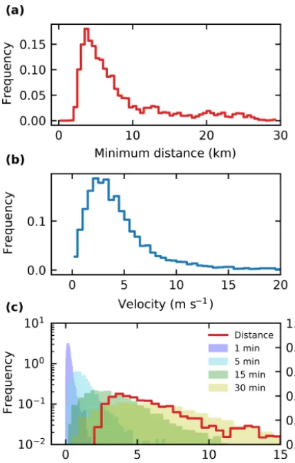
step. Distances between cloudy updrafts (Fig. 5a) were most frequently around 5 km, with a substantial tail of up to 30 km representing more isolated cells. This distribution is indepen-dent of the chosen output time step as it represents an in-stantaneous relationship between cells at individual points in time. The updraft propagation velocities derived for tracking with a 1 min output time step (Fig. 5b) were most frequently at around 4 m s−1, with more than 90 % of the velocities be-low 10 m s−1.

Figure 5. (a)Distributions of the distance to the next identified ob-ject for all identified obob-jects and(b) velocities for tracked cloud objects at each time step of the trajectories.(c)The distribution of derived travel distances of individual clouds during one output time step (shaded colours) resulting from these velocities in(b)is shown together with the distribution of the minimal distance to the nearest neighbour for individual objects as shown in(a).

with 1 min output likely to provide more successful and ac-curate tracks.

The cloud lifetimes (Fig. 6) are analysed for the same 3 h period using the two different time resolutions (1 and 5 min) and agree well for clouds with lifetimes larger than about 15 to 20 min. For shorter lifetimes, the 1 min input data yield substantially more tracked cells. It is obvious that we can only properly represent and analyse cloud lifetimes for clouds that exist over a certain number of output time steps in this framework. An individual cloud that is tracked for 5 to 10 min based on 1 min output allows for robust conclusions about the evolution of the cloud in that period. The same time would merely lead to two or three individually identified ob-jects for 5 min data output, which would be the minimum to draw any useful conclusions about the lifetimes or time evo-lution of the clouds.

Figure 6.Cell lifetimes for tracking and analysis using two different output time steps (1 and 5 min) showing both total counts(a)and the probability distribution function (PDF)(b).

4 Example B: tracking deep convective clouds in model simulations and geostationary satellite data based on outgoing longwave radiation (OLR)

Satellite retrievals are an important tool in climate and weather research as they are an effective way of obtaining observation-based quantities over greater spatial scales in the atmosphere. Specifically, geostationary satellites offer con-tinuous coverage in space and time for a specific region and can therefore be used to understand the temporal evolution of atmospheric phenomena. Direct comparisons of model simu-lations with satellite retrievals for the same area and time pe-riod are an important means of assessing model capabilities to successfully represent atmospheric processes in the real world. Using a tracking framework for the analysis allows us to investigate the representation of clouds in the model in a way that takes the development of individual clouds within the population of clouds into account as opposed to relying on temporal and spatial statistics of the cloud field. Using the same tracking framework for both model and observation data allows for a more robust comparison between them.

The satellite data used in this example have an average hori-zontal spacing of about 4 km.

The model simulation comprises the outermost nested grid of the nested WRF simulation setup described in Sect. 3. This outer domain covers a much larger area, encompass-ing most of Texas and the surroundencompass-ing states of the southern USA, as well as neighbouring areas of northeastern Mex-ico. It features a grid spacing of 4.5 km and a width of 400 grid cells, equivalent to 1800 km in each horizontal direction. The simulation results were output at a time resolution of 15 min for the entire 24 h simulation period from 12:00 UTC on 19 June 2013 to 12:00 UTC on 20 June 2013.

Although the temporal and spatial resolution of the input data can be arbitrary for the use in tobac, a meaningful com-parison of the two datasets requires the analysis to cover the same region at a similar temporal and spatial resolution. The spatial resolution of the two datasets is reasonably similar (around 4 km for the satellite data and 4.5 km for the model output) and both datasets use a regular 15 min interval, with a difference of up to a minute due to the scan time of the satellite data. The satellite data were restricted to the same temporal and spatial extent as the model output.

Top-of-atmosphere outgoing longwave radiation (OLR) is used to track individual deep convective clouds in both model simulations and satellite retrievals. OLR is a standard model output for most high-resolution simulations and is often used as a diagnostic for simulated deep convection (Pearson et al., 2010; Russo et al., 2011). OLR retrievals also have the ben-efit that they do not depend on other aspects of a compli-cated radiative transfer model, which require, amongst other assumptions, pixels to be assigned as either cloud or cloud-free for the radiative retrieval of several optical (effective ra-dius and optical depth) and thermal (cloud-top temperature and height) cloud properties (McGarragh et al., 2018). For the satellite data, we use an empirical conversion derived in Singh et al. (2007) to convert the radiancesLfrom two nels in the GOES-13 measurements, the water vapour chan-nel (WV, 5.8 to 7.30 µm) and a chanchan-nel in the infrared win-dow (WIN, 10.2 to 11.2 µm), to OLR.

OLR=11.44LWIN+9.04LWV+9.11LWV LWIN

−86.36 LWIN

−0.14L2_WV+111.12 (4)

Singh et al. (2007) report an uncertainty from these conver-sions within 2.5 W m−2.

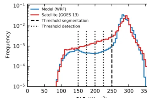
The distribution of OLR for the model simulations and the satellite retrievals shows a very similar shape (Fig. 7). The satellite-retrieved OLR features a larger number of pix-els characterised by lower OLR values in the range between 100 and 250 W m−2corresponding to deep cloud tops. The range covered and the peak position of OLR, correspond-ing to cloud-free and low cloud regions around 290 W m−2, agree well between the model simulation and the satellite re-trieval.

Figure 7.Probability density function of OLR for the model sim-ulation and the satellite retrievals including the thresholds (vertical dashed and dotted lines) set for feature detection and segmentation.

We use these histograms to choose the threshold values for the feature detection and the segmentation steps in the tobac routine. The threshold for the outline of the convective clouds in the segmentation step (250 W m−2) reflects the lower tail of the peak of OLR in both the model simulations and the satellite retrievals. The additional thresholds used in the fea-ture detection algorithm (250, 225, 200, 175 and 150 W m−2) are distributed over the range of OLR values in the part of the distribution representing the deeper clouds.

The individual steps of the tracking analysis for the model data are shown in Fig. 8, but the same steps are applied equally to the satellite-retrieved data. The outgoing long-wave radiation field (Fig. 8a) is filtered with a Gaussian filter with a standard deviation ofσ =4.5 km, equivalent to the grid spacing of the model data (Fig. 8b). The feature iden-tification following Sect. 2.2 is performed with the set of five OLR thresholds of 250, 225, 200, 175 and 150 W m−2 (Fig. 8c, d). The segmentation is performed using the wa-tershedding technique (Sect. 2.3) with an OLR threshold of 250 W m−2to identify the area of the individual clouds lead-ing to the cloud areas shown in Fig. 8e. The complete linked trajectories of all clouds present at the specific time step, as illustrated in the other sub-figures, are shown in Fig. 8f with the cloud extent at the start (dashed) and end (solid) of the lifetime of the cloud.

Figure 8.Schematic overview of the individual steps of the tracking algorithm for an example subset of the domain used in example B based on outgoing longwave radiation. The input data(a)are smoothed with a filter(b)before regions above or below a set of thresholds are determined(c)to identify the individual features(d).(e)The associated cloud areas determined in the segmentation step and(f)all individual clouds present at the time step over their entire life cycle, including an outline of the cloud area at the start (dashed) and at the end (solid) of the trajectory.

tracking analysis and visualisation, is available as a Jupyter notebook as part of the package source code.

The tracked clouds for both the model simulation and the satellite retrieval are visualised for two different times in Fig. 9. Both the model simulations and the satellite retrieval show many individual convective clouds in a region north of the coastline, especially towards the east of the analysed do-main around the Mississippi River Delta and further inland in Texas. In addition, larger connected regions of clouds occur both towards the southern end of the analysed domain over the Gulf of Mexico and in the form of a large organised storm system entering the domain from the northwest. The propa-gation of this large system is not represented accurately in the model simulation, as it shows a lag of several hours and is smaller in magnitude than in the satellite retrievals.

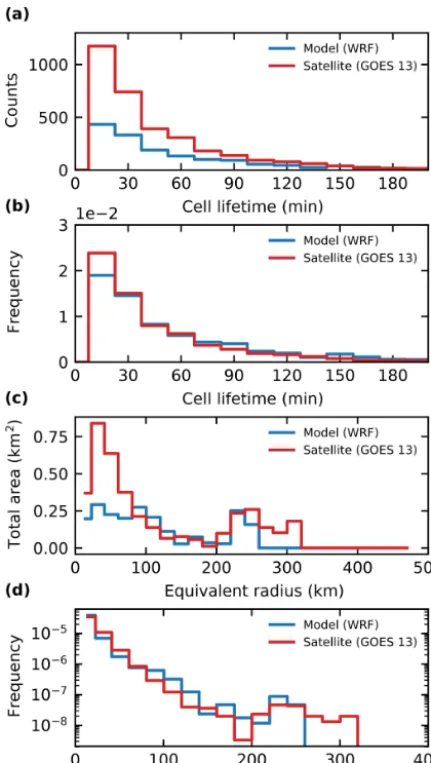
The lifetime distribution of the clouds identified and tracked from the model simulations and from the satellite retrievals shows a similar distribution (see Fig. 10a). How-ever, more clouds are identified in the satellite data than in the model data. When normalised for total number, the life-time distributions agree better between the two different data inputs (Fig. 10b). Most cloud objects are tracked for periods of up to an hour, but in both the model simulations and the satellite retrievals there are numerous cloud objects tracked for up to several hours. The distributions of the cloud areas (Fig. 10c, d) show that the total cloud area for both model and satellite data is made up of two types of identified ob-jects, smaller tracked clouds with a radius of up to 100 km and large tracked features with a radius of a few hundred

kilometres. Due to the larger number of tracked clouds, there is more total cloud area in the tracked clouds in the satellite data. The distribution of cloud sizes is relatively similar be-tween the two datasets. The satellite data show more small clouds below the 100 km equivalent radius. Furthermore, the size of the largest tracked objects is larger in the satellite data than in the model data, which corresponds to the large MCS propagating through the domain of interest (Fig. 9) and which is not represented properly in the model simulations with respect to both timing and total size.

geosta-Figure 9.Identified and tracked objects at two specific points in time (19 June 2013 at 18:55 and 22:55 UTC) based on outgoing longwave radiation for the WRF simulations with 4.5 km grid spacing(a, c)and the outgoing longwave radiation derived from the combination of two GOES-13 channels following Singh et al. (2007)(b, d).

tionary satellite imagers, such as the GOES-R series (GOES 16–17) that has replaced the GOES-13 satellite used here, as well as Himawari-8 (Bessho et al., 2016) and the future Me-teosat Third Generation (MTG) satellites (Stuhlmann et al., 2005), all feature substantially higher temporal and spatial resolution.

The scattered convective cells of differing depths over the area of Houston that were the focus of the analysis in the first application example (Sect. 3) are not clearly resolved in these two datasets. The lower spatial resolution of the simulations and satellite retrieval (around 4 km compared to 500 m in the high-resolution simulations used in Sect. 3) limits the spatial scale of cloud features that can be resolved to more than a few tens of kilometres in radius. The use of outgoing long-wave radiation as a variable for feature identification does not include as much information as the three-dimensional model output fields used in Sect. 3; however, it provides com-plementary information to compare model simulations with satellite retrievals.

5 Conclusions

We have presented tobac, a new framework for the object-based analysis and tracking of individual convective clouds

in different types of input data. The workflow of the soft-ware package consists of the detection of suitable features, segmentation of the areas or volumes representative of an in-dividual cloud object, and subsequent linking of objects at individual time steps into trajectories. All individual steps are implemented in a modular way, thereby allowing for the implementation of different algorithms for each of the steps, should the need arise.

We have developed a feature detection algorithm based on identifying regions above or below a defined sequence of thresholds in two-dimensional input fields. Cloud volumes or cloud areas are associated based on a watershedding tech-nique featuring a single specific threshold value on two- or three-dimensional input fields.

Figure 10.Distributions of cloud lifetimes obtained from the track-ing of model data and satellite retrievals, shown as total counts

(a)and frequency(b). The distribution of cloud areas is shown as the distribution of total area resulting from the sum in each area bin

(d)and as a PDF of cloud area(c). Both these distributions are plot-ted against the equivalent radius of a circular cloud of the same area.

visualisation routines allow for a convenient way to assess the performance of the analysis and evaluate the choice of parameters for the different steps of the analysis framework. The automatically created animated visualisations of individ-ual tracked cells can guide users in the development of fur-ther detailed analyses based on the analysis tools provided in the framework.

The implementation of the tracking framework in Python enables the use of extensive and actively developed open-source libraries for scientific computing. We have shown that this provides numerous advantages, e.g. for memory man-agement, data structures and visualisation. The rapid devel-opment of the underlying libraries means that tobac can profit from future advances without any further development of

to-Figure 11. (a)Distributions of the distance to the next identified object for all identified objects and(b)velocities for tracked cloud objects at each time step of the trajectories for both the model sim-ulations and the satellite data.(d)The travel distance per input in-terval resulting from different time resolution of the input based on these velocities(b) is shown together with the distribution of the minimal distance to the nearest neighbour in(a)for the model data in(c)and for the satellite data.

enable the use of different tracking algorithms in parallel for evaluation and comparisons as well as tracking based on dif-ferent types of input data in a single analysis framework.

We have presented two application examples of the use of tobac for the study of deep convective clouds. In the first ap-plication (example A), we have tracked scattered deep con-vective cells based on a combination of the vertical velocity and total condensate mixing ratio fields from CRM simula-tions with WRF over the area around Houston, Texas. The simulations were performed with a grid spacing of 500 m and thus represent a typical application of a CRM. The track-ing framework is currently betrack-ing applied to other CRMs for the same case study as part of the ACPC deep convection case study (van den Heever et al., 2017) to investigate the response of deep convective clouds in models to changes in aerosols. We have performed the tracking for different out-put frequencies to evaluate the dependency of the tracking performance on the time resolution of the input data. The output resolutions of 1 and 5 min lead to comparable track-ing results for scattered convective cells. This result can be confirmed using an analysis of typical displacement veloci-ties of the clouds and nearest-neighbour distances between the individual identified cloud objects.

In a second application (example B), we have pre-sented a simultaneous tracking of deep convective cloud features and larger convective systems based on outgo-ing longwave radiation output from model simulations with convection-permitting grid spacing (4.5 km) and outgoing longwave radiation derived from geostationary satellite re-trievals (GOES-13) in the same region. The 15 min time res-olution available from the satellite retrieval is shown to be sufficient for successful tracking performance. The analysis also demonstrated that the model simulations and the satel-lite retrieval feature clouds with a similar lifetime distribu-tion. The distribution of cloud areas in model and satellite data shows a similar combination of smaller convective cells and larger systems. The main differences occur for the largest tracked systems, which are stronger in the satellite retrievals. This can be explained by the limited representation of the propagation of two large organised storms within the model domain. This would have been more challenging to assess from a bulk analysis of the domain-wide averaged proper-ties.

The newest generation of geostationary satellites, such as Himawari-8 and GOES-16–17, provide substantially higher spatial and temporal resolution (Bessho et al., 2016; Schmit et al., 2016). These advances will strongly improve the ap-plicability of these types of satellite data for use in object-based tracking and analyses with tobac and also allow for a wider range of applications, e.g. by capturing smaller scat-tered cells such as the ones investigated in Sect. 3.

The ability of tobac to be used for both models and obser-vations as shown in these examples helps to compare models with observations more directly and therefore better under-stand the differences between the two types of data.

Although we have focused on tracking and analysing deep convection here, there are numerous other applications that tobac can be used for without much additional work. There are a large number of existing data products, such as high-resolution radar data, e.g. from NEXRAD over the United States and similar networks in several other regions of the world (Reed et al., 2017), that would be most suited for use with tobac. Furthermore, the application of tobac is not strictly limited to the analysis of clouds, and it can also be applied to study other features of the Earth system that can be identified as well-defined time-evolving regions, such as distinct aerosol plumes in the atmosphere or plankton in the surface layer of the ocean.

We are currently working on implementing additional al-gorithms for the modular steps of the framework, e.g. based on the analyses developed in Senf et al. (2018). Additionally, we are implementing a more flexible representation of the links between cloud objects at specific points in time, which will allow for proper treatment of more complex splitting and merging of cells. We invite the community to contribute to the future development of tobac through the implementation of existing algorithms into the common framework and by using the framework as a basis for new developments.

Code and data availability. The tobac source code is publicly available in a GitHub repository distributed under a BSD 3-Clause licence at https://github.com/climate-processes/tobac (Heikenfeld et al., 2019b, c). The version tobac 1.2 described here is available as a release (Heikenfeld et al., 2019a). The latest version of tobac can be installed using conda with the commandconda install

-c conda-forge tobac.

The linking step makes use oftrackpy(Allan et al., 2016). We use several standard Python packages for scientific computing and image processing that are all available through package managers such as pip or conda. The GOES-13 satellite imager data have been downloaded from the NOAA Comprehensive Large Array- data Stewardship System (CLASS) (NOAA, 2019a) and processed with the NOAA Weather and Climate Toolkit (WCT) (NOAA, 2019b).

Jupyter notebooks containing the tracking analysis and visuali-sations of the tracking results for a smaller subsample of the data used in the two example applications are provided as part of the to-bac source code. The data used in these notebooks are downloaded automatically and are available in Heikenfeld (2019).

Author contributions. MH led the initial development of tobac with contributions by PJM, DWP and FS. MC processed the geostation-ary satellite data and contributed to the analysis of the tracking based on outgoing longwave radiation. MH performed the data anal-ysis and wrote the paper with contributions and approval of the final version by PJM, PS, SCH, MC, DWP and FS.

Acknowledgements. The research has been performed in the frame-work of the IGBP/WCRP initiative ACPC (Aerosols Clouds Precip-itation and Climate) with a focus on developing analysis techniques for the deep convection case study over Houston, Texas. This work used the ARCHER UK National Supercomputing Service and JAS-MIN, the UK collaborative data analysis facility.

Thanks go to William K. Jones and other contributors to the to-bac repository on GitHub for fruitful discussions and contributions to the development of tobac. The authors would like to thank two anonymous reviewers for their useful comments during the review stage of this paper.

Financial support. Max Heikenfeld acknowledges funding from the NERC Oxford DTP in Environmental Research (grant no. NE/L002612/1). The research leading to these results has re-ceived funding from the European Union’s Seventh Framework Pro-gramme (grant no. FP7/2007-2013) project BACCHUS under grant agreement no. 603445 and the European Research Council under the European Union’s Horizon 2020 research and innovation pro-gramme with grant agreement no. 724602 (RECAP). Susan C. van den Heever and Peter J. Marinescu acknowledge funding from the NASA CAMPEx project under grant 80NSSC18K0149, and Peter J. Marinescu was also partially funded by National Science Foun-dation Graduate Research Fellowship grant DGE-1321845. Fabian Senf acknowledges funding within the High Definition Clouds and Precipitation for advancing Climate Prediction (HD(CP)2) project funded by the BMBF (German Ministry for Education and Re-search) under grant 01LK1507C.

Review statement. This paper was edited by Paul Ullrich and re-viewed by two anonymous referees.

References

Allan, D., Caswell, T., Keim, N., and van der Wel, C.: Trackpy, Zenodo, https://doi.org/10.5281/zenodo.1213240, 2019. Autonès, F. and Moisselin, J. M.: Algorithm Theoretical Basis

Doc-ument for “Rapid Development Thunderstorms” (RDT-PGE11 v3.0), Tech. rep., SAF/NWC/CDOP/MFT/SCI/ATBD/11, available at: http://www.nwcsaf.org/AemetWebContents/ ScientificDocumentation/Documentation/MSG/

SAF-NWC-CDOP2-MFT-SCI-ATBD-11_v3.0.pdf (last ac-cess: 19 October 2019), 2013.

Bacmeister, J. T. and Stephens, G. L.: Spatial Statistics of Likely Convective Clouds in CloudSat Data, J. Geophys. Res.-Atmos., 116, D04104, https://doi.org/10.1029/2010JD014444, 2011. Bessho, K., Date, K., Hayashi, M., Ikeda, A., Imai, T.,

In-oue, H., Kumagai, Y., Miyakawa, T., Murata, H., Ohno, T., Okuyama, A., Oyama, R., Sasaki, Y., Shimazu, Y., Shimoji, K., Sumida, Y., Suzuki, M., Taniguchi, H., Tsuchiyama, H., Uesawa, D., Yokota, H., and Yoshida, R.: An Introduction to Himawari-8/9 – Japan’s New-Generation Geostationary Meteo-rological Satellites, J. Meteorol. Soc. JPN, Ser. II, 94, 151–183, https://doi.org/10.2151/jmsj.2016-009, 2016.

CEDA: JASMIN, the UK Collaborative Data Analysis Facility, available at: http://jasmin.ac.uk/ (last access: 19 October 2019), 2019.

Chen, Q., Koren, I., Altaratz, O., Heiblum, R. H., Dagan, G., and Pinto, L.: How do changes in warm-phase microphysics affect deep convective clouds?, Atmos. Chem. Phys., 17, 9585–9598, https://doi.org/10.5194/acp-17-9585-2017, 2017.

Cotton, W. R., Bryan, G., and van den Heever, S. C.: Storm and Cloud Dynamics, Academic Press, 2010.

Couvreux, F., Hourdin, F., and Rio, C.: Resolved Ver-sus Parametrize Boundary-Layer Plumes. Part I: A Parametrization-Oriented Conditional Sampling in Large-Eddy Simulations, Bound.-Lay. Meteorol., 134, 441–458, https://doi.org/10.1007/s10546-009-9456-5, 2010.

Crane, R.: Automatic Cell Detection and Track-ing, IEEE Trans. Geosci. Electro., 17, 250–262, https://doi.org/10.1109/TGE.1979.294654, 1979.

Crocker, J. C. and Grier, D. G.: Methods of Digital Video Mi-croscopy for Colloidal Studies, J. Colloid Interf. Sci., 179, 298– 310, https://doi.org/10.1006/jcis.1996.0217, 1996.

Dask Development Team: Dask: Library for Dynamic Task Scheduling, available at: https://dask.org (last access: 19 Octo-ber 2019), 2016.

Davis, C., Brown, B., and Bullock, R.: Object-Based Verifica-tion of PrecipitaVerifica-tion Forecasts. Part II: ApplicaVerifica-tion to Con-vective Rain Systems, Mon. Weather Rev., 134, 1785–1795, https://doi.org/10.1175/MWR3146.1, 2006.

Davis, C. A., Brown, B. G., Bullock, R., and Halley-Gotway, J.: The Method for Object-Based Diagnostic Evaluation (MODE) Applied to Numerical Forecasts from the 2005 NSSL/SPC Spring Program, Weather Forecast., 24, 1252–1267, https://doi.org/10.1175/2009WAF2222241.1, 2009.

Dawe, J. T. and Austin, P. H.: Statistical analysis of an LES shallow cumulus cloud ensemble using a cloud tracking algorithm, At-mos. Chem. Phys., 12, 1101–1119, https://doi.org/10.5194/acp-12-1101-2012, 2012.

Dixon, M. and Wiener, G.: TITAN: Thunderstorm Identification, Tracking, Analysis, and Nowcasting – A Radar-Based Methodology, J. Atmos. Ocean. Technol., 10, 785–797, https://doi.org/10.1175/1520-0426(1993)010<0785:TTITAA>2.0.CO;2, 1993.

Doswell, C. A.: Severe Convective Storms – An Overview, in: Se-vere Convective Storms, edited by: Doswell, C. A., Meteoro-logical Monographs, 1–26, Am. Meteorol. Soc., Boston, MA, https://doi.org/10.1007/978-1-935704-06-5_1, 2001.

Emanuel, K. A.: Atmospheric Convection, Oxford University Press, New York, 1994.

Fan, J., Han, B., Varble, A., Morrison, H., North, K., Kol-lias, P., Chen, B., Dong, X., Giangrande, S. E., Khain, A., Lin, Y., Mansell, E., Milbrandt, J. A., Stenz, R., Thomp-son, G., and Wang, Y.: Cloud-Resolving Model Intercom-parison of an MC3E Squall Line Case: Part I – Con-vective Updrafts, J. Geophys. Res.-Atmos., 122, 9351–9378, https://doi.org/10.1002/2017JD026622, 2017.

Feng, Z., Leung, L. R., Houze Jr., R. A., Hagos, S., Hardin, J., Yang, Q., Han, B., and Fan, J.: Structure and Evolu-tion of Mesoscale Convective Systems: Sensitivity to Cloud Microphysics in Convection-Permitting Simulations Over the United States, J. Adv. Model. Earth Syst., 10, 1470–1494, https://doi.org/10.1029/2018MS001305, 2018.

Fiolleau, T. and Roca, R.: An Algorithm for the Detec-tion and Tracking of Tropical Mesoscale Convective Sys-tems Using Infrared Images From Geostationary Satel-lite, IEEE Trans. Geosci. Remote Sens., 51, 4302–4315, https://doi.org/10.1109/TGRS.2012.2227762, 2013.

Fritsch, J. M. and Forbes, G. S.: Mesoscale Convective Systems, in: Severe Convective Storms, edited by: Doswell, C. A., Mete-orological Monographs, 323–357, Am. Meteorol. Soc., Boston, MA, https://doi.org/10.1007/978-1-935704-06-5_9, 2001. Fu, H., Shen, Y., Liu, J., He, G., Chen, J., Liu, P., Qian, J., and

Li, J.: Cloud Detection for FY Meteorology Satellite Based on Ensemble Thresholds and Random Forests Approach, Remote Sens., 11, 44, https://doi.org/10.3390/rs11010044, 2019. Gensini, V. A. and Mote, T. L.: Estimations of Hazardous

Convec-tive Weather in the United States Using Dynamical Downscaling, J. Climate, 27, 6581–6589, https://doi.org/10.1175/JCLI-D-13-00777.1, 2014.

Grady, L.: Random Walks for Image Segmentation, IEEE Trans. Pattern Anal. Machine Intell., 28, 1768–1783, https://doi.org/10.1109/TPAMI.2006.233, 2006.

Guillaume, A., Kahn, B. H., Yue, Q., Fetzer, E. J., Wong, S., Ma-nipon, G. J., Hua, H., and Wilson, B. D.: Horizontal and Verti-cal SVerti-caling of Cloud Geometry Inferred from CloudSat Data, J. Atmos. Sci., 75, 2187–2197, https://doi.org/10.1175/JAS-D-17-0111.1, 2018.

Hagos, S., Feng, Z., McFarlane, S., and Leung, L. R.: Environ-ment and the Lifetime of Tropical Deep Convection in a Cloud-Permitting Regional Model Simulation, J. Atmos. Sci., 70, 2409– 2425, https://doi.org/10.1175/JAS-D-12-0260.1, 2013.

Heiblum, R. H., Altaratz, O., Koren, I., Feingold, G., Kostinski, A. B., Khain, A. P., Ovchinnikov, M., Fredj, E., Dagan, G., Pinto, L., Yaish, R., and Chen, Q.: Characterization of Cumu-lus Cloud Fields Using Trajectories in the Center of Gravity versus Water Mass Phase Space: 2. Aerosol Effects on Warm Convective Clouds, J. Geophys. Res.-Atmos., 121, 6356–6373, https://doi.org/10.1002/2015JD024193, 2016a.

Heiblum, R. H., Altaratz, O., Koren, I., Feingold, G., Kostinski, A. B., Khain, A. P., Ovchinnikov, M., Fredj, E., Dagan, G., Pinto, L., Yaish, R., and Chen, Q.: Characterization of Cumu-lus Cloud Fields Using Trajectories in the Center of Gravity versus Water Mass Phase Space: 1. Cloud Tracking and Phase Space Description, J. Geophys. Res.-Atmos., 121, 6336–6355, https://doi.org/10.1002/2015JD024186, 2016b.

Heikenfeld, M.: Tobac Example Datasets, https://doi.org/10.5281/zenodo.3195909, 2019.

Heikenfeld, M., Jones, W. K., Senf, F., and Marinescu, P. J.: To-bac 1.2: Tracking and Object-Based Analysis of Clouds, Zenodo, https://doi.org/10.5281/zenodo.3408268, 2019a.

Heikenfeld, M., Jones, W. K., Senf, F., and Marinescu, P. J.: To-bac: Tracking and Object-Based Analysis of Clouds, available at: https://github.com/climate-processes/tobac (last access: 19 Octo-ber 2019), 2019b.

Heikenfeld, M., Jones, W. K., Senf, F., and Marinescu, P. J.: To-bac: Tracking and Object-Based Analysis of Clouds, Zenodo, https://doi.org/10.5281/zenodo.2577046, 2019c.

Hernandez-Deckers, D. and Sherwood, S. C.: A Numerical Inves-tigation of Cumulus Thermals, J. Atmos. Sci., 73, 4117–4136, https://doi.org/10.1175/JAS-D-15-0385.1, 2016.

Heus, T. and Seifert, A.: Automated tracking of shallow cumulus clouds in large domain, long duration large eddy simulations, Geosci. Model Dev., 6, 1261–1273, https://doi.org/10.5194/gmd-6-1261-2013, 2013.

Heus, T., Jonker, H. J. J., Van den Akker, H. E. A., Griffith, E. J., Koutek, M., and Post, F. H.: A Statistical Approach to the Life Cycle Analysis of Cumulus Clouds Selected in a Virtual Reality Environment, J. Geophys. Res.-Atmos., 114, D06208, https://doi.org/10.1029/2008JD010917, 2009.

Hillger, D. W. and Schmit, T. J.: The GOES-13 Science Test: Im-ager and Sounder Radiance and Product Validations, NOAA, En-viron. Satell. Data Inf. Serv., Silver Spring, MD, NOAA Tech. Rep, 141, 2007.

Hoyer, S. and Hamman, J.: Xarray: N-D Labeled Arrays and Datasets in Python, J. Open Res. Softw., 5, 10, https://doi.org/10.5334/jors.148, 2017.

Hunter, J. D.: Matplotlib: A 2D Graphics Environment, Com-put. Sci. Eng., 9, 90–95, https://doi.org/10.1109/MCSE.2007.55, 2007.

Iacono, M. J., Delamere, J. S., Mlawer, E. J., Shephard, M. W., Clough, S. A., and Collins, W. D.: Radiative Forcing by Long-Lived Greenhouse Gases: Calculations with the AER Radia-tive Transfer Models, J. Geophys. Res.-Atmos., 113, D13103, https://doi.org/10.1029/2008JD009944, 2008.

Igel, M. R., Drager, A. J., and van den Heever, S. C.: A Cloud-Sat Cloud Object Partitioning Technique and Assessment and Integration of Deep Convective Anvil Sensitivities to Sea Sur-face Temperature, J. Geophys. Res.-Atmos., 119, 10515–10535, https://doi.org/10.1002/2014JD021717, 2014.

IPCC: Climate Change 2013: The Physical Science Basis. Contri-bution of Working Group I to the Fifth Assessment Report of the Intergovernmental Panel on Climate Change, Cambridge Uni-versity Press, Cambridge, United Kingdom and New York, NY, USA, https://doi.org/10.1017/CBO9781107415324, 2013. Kluyver, T., Ragan-Kelley, B., Pérez, F., Granger, B. E., Bussonnier,

M., Frederic, J., Kelley, K., Hamrick, J. B., Grout, J., and Corlay, S.: Jupyter Notebooks – a Publishing Format for Reproducible Computational Workflows., in: ELPUB, 87–90, 2016.

Laing, A. G. and Fritsch, J. M.: The Global Population of Mesoscale Convective Complexes, Q. J. Roy. Meteorol. Soc., 123, 389–405, https://doi.org/10.1002/qj.49712353807, 1997.

Lakshmanan, V. and Smith, T.: An Objective Method of Evaluating and Devising Storm-Tracking Algorithms, Weather Forecast., 25, 701–709, https://doi.org/10.1175/2009WAF2222330.1, 2009. Liang, K., Shi, H., Yang, P., and Zhao, X.: An Integrated Convective

Cloud Detection Method Using FY-2 VISSR Data, Atmosphere, 8, 42, https://doi.org/10.3390/atmos8020042, 2017.

Lin, J. W.-B.: Why Python Is the Next Wave in Earth Sci-ences Computing, B. Am. Meteorol. Soc., 93, 1823–1824, https://doi.org/10.1175/BAMS-D-12-00148.1, 2012.

Rev., 126, 1630–1654, https://doi.org/10.1175/1520-0493(1998)126<1630:LCVOMC>2.0.CO;2, 1998.

McGarragh, G. R., Poulsen, C. A., Thomas, G. E., Povey, A. C., Sus, O., Stapelberg, S., Schlundt, C., Proud, S., Christensen, M. W., Stengel, M., Hollmann, R., and Grainger, R. G.: The Com-munity Cloud retrieval for CLimate (CC4CL) – Part 2: The op-timal estimation approach, Atmos. Meas. Tech., 11, 3397–3431, https://doi.org/10.5194/amt-11-3397-2018, 2018.

McKinney, W.: Data Structures for Statistical Computing in Python, in: Proceedings of the 9th Python in Science Conference, 51–56, available at: http://conference.scipy.org/proceedings/scipy2010/ mckinney.html (last access: 19 October 2019), 2010.

Mecikalski, J. R. and Bedka, K. M.: Forecasting Convective Ini-tiation by Monitoring the Evolution of Moving Cumulus in Daytime GOES Imagery, Mon. Weather Rev., 134, 49–78, https://doi.org/10.1175/MWR3062.1, 2006.

Mecikalski, J. R., Watts, P. D., and Koenig, M.: Use of Meteosat Second Generation Optimal Cloud Anal-ysis Fields for Understanding Physical Attributes of Growing Cumulus Clouds, Atmos. Res., 102, 175–190, https://doi.org/10.1016/j.atmosres.2011.06.023, 2011.

Menzel, W. P.: Cloud Tracking with Satellite Imagery: From the Pioneering Work of Ted Fujita to the Present, B. Am. Meteorol. Soc., 82, 33–48, https://doi.org/10.1175/1520-0477(2001)082<0033:CTWSIF>2.3.CO;2, 2001.

Met Office: Iris: A Python Library for Analysing and Visualising Meteorological and Oceanographic Data Sets, Tech. rep., 2018. Meyer, F.: Topographic Distance and Watershed Lines, Signal Proc.,

38, 113–125, https://doi.org/10.1016/0165-1684(94)90060-4, 1994.

Morrison, H., Curry, J. A., and Khvorostyanov, V. I.: A New Double-Moment Microphysics Parameterization for Application in Cloud and Climate Models. Part I: Description, J. Atmos. Sci., 62, 1665–1677, https://doi.org/10.1175/JAS3446.1, 2005. Morrison, H., Thompson, G., and Tatarskii, V.: Impact of Cloud

Microphysics on the Development of Trailing Stratiform Pre-cipitation in a Simulated Squall Line: Comparison of One- and Two-Moment Schemes, Mon. Weather Rev., 137, 991–1007, https://doi.org/10.1175/2008MWR2556.1, 2009.

Moseley, C., Berg, P., and Haerter, J. O.: Probing the Precipitation Life Cycle by Iterative Rain Cell Track-ing, J. Geophys. Res.-Atmos., 118, 13361–13370, https://doi.org/10.1002/2013JD020868, 2013.

Moseley, C., Hohenegger, C., Berg, P., and Haerter, J. O.: Intensification of Convective Extremes Driven by Cloud-Cloud Interaction, Nat. Geosci., 9, 748–752, https://doi.org/10.1038/ngeo2789, 2016.

NCEP: NCEP GDAS/FNL 0.25 Degree Global Tro-pospheric Analyses and Forecast Grids, Tech. rep., https://doi.org/10.5065/D65Q4T4Z, 2015.

Nesbitt, S. W., Zipser, E. J., and Cecil, D. J.: A Census of Precipitation Features in the Tropics Using TRMM: Radar, Ice Scattering, and Lightning Observations, J. Climate, 13, 4087–4106, https://doi.org/10.1175/1520-0442(2000)013<4087:ACOPFI>2.0.CO;2, 2000.

Nesbitt, S. W., Cifelli, R., and Rutledge, S. A.: Storm Morphology and Rainfall Characteristics of TRMM Precipitation Features, Mon. Weather Rev., 134, 2702–2721, 2006.

NOAA: NOAA’s Comprehensive Large Array-Data Stewardship System – GOES Satellite Data – Imager (GVAR_IMG), avail-able at: https://www.avl.class.noaa.gov/saa/products/search? datatype_family=GVAR_IMG (last access: 19 October 2019), 2019a.

NOAA: NOAA Weather and Climate Toolkit (WCT), National Cli-matic Data Center, NESDIS, NOAA, available at: https://www. ncdc.noaa.gov/wct/ (last access: 19 October 2019), 2019b. O’Brien, T. A., Li, F., Collins, W. D., Rauscher, S. A., Ringler,

T. D., Taylor, M., Hagos, S. M., and Leung, L. R.: Observed Scaling in Clouds and Precipitation and Scale Incognizance in Regional to Global Atmospheric Models, J. Climate, 26, 9313– 9333, https://doi.org/10.1175/JCLI-D-13-00005.1, 2013. Orlanski, I.: A Rational Subdivision of Scales for

Atmo-spheric Processes, B. Am. Meteorol. Soc., 56, 527–530, https://doi.org/10.1175/1520-0477-56.5.527, 1975.

Pearson, K. J., Hogan, R. J., Allan, R. P., Lister, G. M. S., and Holloway, C. E.: Evaluation of the Model Representation of the Evolution of Convective Systems Using Satellite Observations of Outgoing Longwave Radiation, J. Geophys. Res.-Atmos., 115, D20206, https://doi.org/10.1029/2010JD014265, 2010. Perez, F. and Granger, B. E.: IPython: A System for

Inter-active Scientific Computing, Comput. Sci. Eng., 9, 21–29, https://doi.org/10.1109/MCSE.2007.53, 2007.

Perkel, J. M.: Programming: Pick up Python, Nat. News, 518, 125, https://doi.org/10.1038/518125a, 2015.

Plant, R. S.: Statistical properties of cloud lifecycles in cloud-resolving models, Atmos. Chem. Phys., 9, 2195–2205, https://doi.org/10.5194/acp-9-2195-2009, 2009.

Reed, J. L., Lanterman, A. D., and Trostel, J. M.: Weather Radar: Operation and Phenomenology, IEEE Aero. Elect. Syst. Magaz., 32, 46–62, https://doi.org/10.1109/MAES.2017.150178, 2017. Riley, E. M., Mapes, B. E., and Tulich, S. N.: Clouds

Asso-ciated with the Madden – Julian Oscillation: A New Per-spective from CloudSat, J. Atmos. Sci., 68, 3032–3051, https://doi.org/10.1175/JAS-D-11-030.1, 2011.

Rocklin, M.: Dask: Parallel Computation with Blocked Algorithms and Task Scheduling, in: Proceedings of the 14th Python in Sci-ence ConferSci-ence, edited by: Huff, K. and Bergstra, J., 130–136, 2015.

Rosenfeld, D.: Objective Method for Analysis and Track-ing of Convective Cells as Seen by Radar, J. Atmos. Ocean. Technol., 4, 422–434, https://doi.org/10.1175/1520-0426(1987)004<0422:OMFAAT>2.0.CO;2, 1987.

Russo, M. R., Marécal, V., Hoyle, C. R., Arteta, J., Chemel, C., Chipperfield, M. P., Dessens, O., Feng, W., Hosking, J. S., Telford, P. J., Wild, O., Yang, X., and Pyle, J. A.: Representa-tion of tropical deep convecRepresenta-tion in atmospheric models – Part 1: Meteorology and comparison with satellite observations, At-mos. Chem. Phys., 11, 2765–2786, https://doi.org/10.5194/acp-11-2765-2011, 2011.

Schmit, T. J., Griffith, P., Gunshor, M. M., Daniels, J. M., Good-man, S. J., and Lebair, W. J.: A Closer Look at the ABI on the GOES-R Series, B. Am. Meteorol. Soc., 98, 681–698, https://doi.org/10.1175/BAMS-D-15-00230.1, 2016.