Volume 17, Number 4 (2019), 517-529
URL:https://doi.org/10.28924/2291-8639 DOI:10.28924/2291-8639-17-2019-517
BIFURCATIONS AND INVARIANT SETS IN A CLASS OF TWO-DIMENSIONAL ENDOMORPHISMS
DJELLIT ILHAM1,∗, FAKROUNE YAMINA1 AND SELMANI WISSAME2
1Laboratory of Mathematics, Dynamics and Modelization, University Badji Mokhtar, Annaba-Algeria
2University 20 Aout 1955, Skikda-Algeria
∗Corresponding author: [email protected]
Abstract. Several endomorphisms of the plane have been constructed by simple maps. We study the dynamics occuring in one of them, which is rich in global bifurcations. The invariants sets are stable manifolds of saddle type points or cycles, as well as closed curves issued from Hopf bifurcations. The present paper focuses some bifurcations related with attractors or basins which produce other attractors which coexist with invariant sets.
1. Introduction
Multistable systems, i.e. systems with a large number of coexisting stable systems, are very common in
nature. They are subject of increasing interest in the last two decades. It has been the discovery of multiple
stable states in many systems (Agarwal in [1]; Arecchi et al. in [2]; Djellit and Soula in [4]) that triggered
the research in many other fields. Multistable behaviors were found in discrete systems (H´enon in [9]; Ikeda
in [10]; Grebogi et al. in [7]; Feudel et al. in [6]; Lorenz in [11]).
We present and explain numerical results illustrating the mechanism of bifurcations that occurs in a
typical dynamical system relative to ”coupled-uncoupled” two-dimensional map. Because the non-unique
dynamics associated with the degree of the nonlinearity leads to a real interest and a large richness of the
Received 2019-03-25; accepted 2019-04-22; published 2019-07-01. 2010Mathematics Subject Classification. 37G10, 37J20, 37J15, 37D10. Key words and phrases. bifurcation; endomorphism; attractor.
c
2019 Authors retain the copyrights
of their papers, and all open access articles are distributed under the terms of the Creative Commons Attribution License.
bifurcations situations, and interesting phenomena are uncovered, due in essence to the presence of invariant
sets. This can have a profound effect on our understanding of the dynamical behavior. We provide numerical
evidence and show some mechanisms associated with the appearance and disappearance of closed invariant
curves.
Consider this dynamical system generated by a family of two-dimensional continuous noninvertible maps
Ta,b defined by :
Ta,b:
x0 =y
y0=ay−bx+x2
(1)
Fora= 1 andbreal parameter, this map was already studied by Razafimandimby [14] and in Clerc and
Hartmann [3]. They considered the influence domains of stable singularities of the quadratic endomorphism
and they studied self-intersections of the unstable set in the form of loops. This fact has fundamental and
known consequences in bifurcations theory particularly in global bifurcations and chaos. Such bifurcations
governing the route to chaos have been extensively studied since 1975 in [8,12].
Many of chaotic behaviors that are observed in dynamical systems are intimately associated with the
pres-ence of homoclinic and/or heteroclinic points of maps. Contact bifurcations may correspond to homoclinic
and heteroclinic bifurcations, critical and /or invariant curves are useful for interpreting such problems.
Sev-eral papers have shown the importance of critical curves in the bifurcations of basins, for example Gumowski
and Mira [8] who have developed the role of these curves in bifurcations from simply connected basin to
nonconnected basin, Ferchichi et al. in [5] and Mira et al. in [13] have studied bifurcations of type Simply
connected basin to multiply connected basin. These basic bifurcations result from the contact of a basin
boundary with a critical curve segment or an attracting set leading to modifications of the basin.
We study an endomorphism using both analytic bifurcation theory and numerical methods. The dynamics
involves various transitions by bifurcations. The analysis of the dynamics of this model as a function of three
parameters (a, b,andn) is not an easy task. The particular case, witha= 1 fixed, as a function of (b, n= 2)
has been studied in Ref. [3]. There it has been shown that for the mapT, the bifurcations of the model and
route to chaos could be well determined.
The planar system is the following:
Ta,b,n :
x0=y
y0 =ay+fn(x)
(2)
where x, y are real variables,a and b are real parameters. Ta,b,n has a nonconstant Jacobian determinant
detJ =−fn0(x).
These systems Ta,b,n which become uncoupled when a = 0, are of fundamental importance in dynamical
curves : two well-established methods. We display invariant sets for n = 2,and 4 and we examine their
properties. We mainly focused on this research area, the identification and verification of some properties of
such maps.
First we consider the structure of the one-dimensional endomorphism of then-degree polynomial
fn(x) =xn−bx=x(xn−1−b) (3)
wherefn(x) is assumed to depend continuously on the real parameterb.
Forneven,n= 2k, k>1, the fixed points offnare : x= 0 a stable node forb∈]−1; 1[ andx1= (b+ 1)
1
n−1
stable node forb∈]n+1
n−1;−1[.
Forn= 2k+ 1,the equationfn(x) =xadmits a unique trivial solutionx= 0 forb≤ −1: and forb >−1;we
have three solutionsx= 0;x1= (b+ 1)
1
n−1, andx2=−(b+ 1)n−11.
For n= 2 , the two-dimensional endomorphism (2) has some symmetry property and possesses at most 2
fixed points depending upon the parameter values. We describe a specific family of bifurcations in a region
of real parameter plane (a, b) for which the mappings were expected to have simple dynamics. We compute
the first few bifurcation curves in this family and we study the bifurcation diagram which consists to these
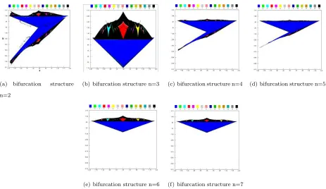
bifurcation curves in the parameter (a, b) plane. The Figures 1.(a, b, c, d, e, f) give the parameter value for
which at least one fixed point is attractive (blue domain corresponding to the value 1). More generally, these
figures give the existence domains of a stable cycle of orderkof which is given by the upper colored squares.
The black regions (k= 15) corresponds to the existence of bounded iterated sequences. These figures are
typical of maps with dominating odd or even degree terms.We can recognize on the diagram period doubling
bifurcations, and spring area communication according to Mira [13]. The bifurcation structure is a ”
box-within-a-box ” type, as is well known infinitely many periodic are opened by fold bifurcations and are closed
by homoclinic bifurcations by the intriguing ” box-within-a-box ” bifurcation structure. When n is even,
there is an interesting passage from symmetric parameter diagram to non symmetric parameter diagram
(clearly visible for the existence domain related with fixed points of color blue). And we can remark that for
neven or odd, the diagrams are quite similar and then we can argue that some properties are automatically
deduced. For n = 2, the two existence domains associated with the two fixed points are symmetric with
respect to a black line located in the frontier to each domain, for n even or odd, the existence domains of
different k-cycles shrink. Forn = 3, the two domains are superimposed and symmetric to the linea= 0.
This case (nodd) is treated separately in an other paper.
Despite the simplicity of this map, the concept ”coupled-uncoupled” is central to our interest and subject.
So, in the following we shall focus our attention on the description of the bifurcations which are expected to
(a) bifurcation structure n=2
(b) bifurcation structure n=3 (c) bifurcation structure n=4 (d) bifurcation structure n=5
(e) bifurcation structure n=6 (f) bifurcation structure n=7
Figure 1. Bifurcation structure for n even and odd values.
This paper intends to give such a study, particularly to consider the map (2) with n = 2. Therefore, it
is structured in the following way. In Section 2 we introduce the language used in [12,13];to analyze the
system, and give some properties. Section 3 gives some results concerning the uncoupled map and the main
bifurcations. Section 4 illustrates properties of invariant curves and connected-nonconnected bifurcation
basins.
2. Symmetry and fundamental properties
First we analyse the dynamics for the caseT =Ta,b,2of the form
Ta,b,2(x, y) = (y, ay+f2(x))
with f2(x) =x2−bx, aand b are real parameters. Let us consider the case f2(x) a quadratic polynomial
(n= 2). We know some results which enable us to detect, predict, determine cycles and fixed points, and
locate bifurcation curves in the parameter plane.
The fixed points and basic bifurcations of Ta,b,2 were analyzed, they are solutions obtained by a trivial
manipulation withx0=xandy0=y: Besides the trivial solutionO(0; 0), we can observe that further fixed
pointP(1 +b−a,1 +b−a) exists ifa6= 1 +b.
In this section we focus our attention on bifurcations playing an important role in the dynamics, those
Proposition 2.1. : If b=−1 +a, then O(0; 0) is the unique fixed point of the map Ta,b,2 defined by (1). The parameter curveΛ(1)0 :b=−1 +ais the transcritical bifurcation curve such that the two fixed pointsO
andP exist, and are symmetric with respect to the parameter curve.
Consider the variable change that moves the pointP to coincide with the origin as follows
x=x∗+ 1 +b−a
y=y∗+ 1 +b−a
.
After injection of this change inT(=Ta,b,2) and some simple simplification, we have
x∗=y∗
y=ay∗−x∗∗x∗−(2a−b−2)x∗
We putb∗ = 2a−b−2, anda∗=a,Ta,b,2becomes Ta∗,b∗,2.
To simplify the notation, in the following we shall write T∗instead ofTa∗,b∗,2. This new mapT∗ has two
fixed points (0,0) which corresponds toP forT and P∗(1 +b∗−a∗,1 +b∗−a∗) which corresponds to the
trivial solution forT.These two mapsT andT∗ change their fixed points.
LetL: R 2→
R2
(x, y)(a,b)→(x∗, y∗)(a∗,b∗)= (x−(1 +b−a), y−(1 +b−a))(a,2a−b−2)
.
Proposition 2.2. L is symmetric by respect to∆, orL◦T =T∗◦L.
Corollary 2.1. If P is a fixed point ofT, thenL(P)is a fixed point of T∗.
Corollary 2.2. The parametric curve Λ(1)0 :b=−1 +ais invariant byL.
The fixed point P(1 +b−a,1 +b−a) with the parametric vector (a, b) is associated with the fixed point
O(0,0)(a∗,b∗) related to parametric vector (a∗, b∗) = (a,2a−b−2). Thus both fixed point O and P can
undergo identical sets of bifurcations in parameter space. We can choose the parameters so that one fixed
point experiences all the bifurcations, while the other has none. It suffices then to study the nature and
bifurcations ofO(0,0) ; those ofP are deduced automatically.
J = 0 1
−b+ 2x a
,
We consider now the conditions of local stability of the fixed pointO(0; 0), in terms of the parameters of
the mapT.
WithJ(0,0)=
0 1
−b a
, is Jacobian matrix ofT in O(0; 0) which has two eigenvalues λ1 = a2 +
q
a2
4 −b;
λ2=a2 −
q
a2
4 −b. We can conclude fora
2−4b >0 with consideringb < a2
4 :
Proof. Consider the square mapT2(the second iterate ofT) : T2(x;y) = T(y, ay−bx+x2) = (ay−bx+
x2, a(ay−bx+x2)−by+y2).
Fixed points of T2 are computed by considering T2(x, y) = (x, y),we obtain then : ay−bx+x2 = xand
a(ay−bx+x2)−by+y2=y.We put from the first equationy= ((1 +b)x−x2)/a, and by replacingy with
its value in the second equation we obtain a quartic polynomial of x. After simplification of the two fixed
points, we have this quadratic polynomial : Q(x) =x2−(1 +a+b)x+a(1 +a+b).Roots ofQ(x) are the
abscissa of the two points of the cycle of order 2 : x1,2= ((1 +a+b)±
p
(1 +a+b)(1 +b−3a))/2 and the
ordinates are : y1=x2 ;y2=x1.
The sufficient condition for the existence of the 2-cycle is given by (1 +a+b)(1 +b−3a)>0.If (1 +a+
b)(1 +b−3a) = 0 we have a flip bifurcation.
Let us denote :
Λ1=
a
b
/ 1 +a+b= 0
and Λ01=
a
b
/ 1 +b−3a= 0
If 1 +a+b= 0 we havex1=x2= 0, this flip bifurcation line Λ1 is associated with the fixed pointO(0,0).
If 1 +b−3a= 0 we havex1=x2= 2a,this flip bifurcation line Λ 0
1is associated with the other fixed point
P(1 +b−a,1 +b−a).
Also the two curves Λ1 and Λ 0
1 are clearly visible in Figure 1.(a).
Proposition 2.4. The map T undergoes discrete Hopf bifurcations at the fixed point O(0,0) fora= 2cos
(αk)andb= 1.
Proof. We obtain the parameter values related to Hopf bifurcations for the fixed pointO(0,0) of focus type
if we put the eigenvaluesλ1= exp(iαk) andλ2= exp(−iαk) withαk =2kπ;k∈N.
Proposition 2.5. The parametric lineb−2a+ 3 = 0is the symmetric of the line ∆ :b= 1with respect to the lineΛ(1)0:b−a+ 1 = 0.
This line∆0 :b−2a+ 3 = 0is associated with the fixed pointP and plays a key role for global bifurcations.
Similarly for ∆ which is associated with the trivial fixed pointO for global bifurcations.
Proof. With a simple computation we obtain this line.
From Fig1.(a), we can see that the stability domain of the trivial fixed pointO = (0,0) is represented
by a blue triangle, bounded by the transcritical bifurcation curve Λ(1)0 :b−a+ 1 = 0, the flip bifurcation
curve 1 +a+b= 0 and the Hopf bifurcation curve ∆ :b= 1. And for the fixed pointP(1 +b−a,1 +b−a)
another blue triangle is associated, bounded by the transcritical bifurcation curve ∆0:b−a+ 1 = 0, the flip
3. Uncoupled map properties
Fora= 0, the second iterate of the map, i.e. T2 is a uncoupled map becauseT2(x;y) =T(y,−bx+x2) =
(−bx+x2,−by+y2) = (f
2(x), f2(y)) is with separate variables.Then, the dynamics of T is associated with
those off2and their bifurcations also are strictly related. If we consider thenf2(x) =−bx+x2,its derivative
isf20(x) =−b+ 2x.For−3< b <−1 : f2 has two points, the trivial pointx= 0 which is unstable with an
eigenvalue equal tob, and the other pointb+ 1 stable and its eigenvalue is equal tob+ 2.
AlsoT has two fixed pointsO= (0; 0) etP = (b+ 1;b+ 1). The first point is a saddle with eigenvalues
λ1,2=± √
−b. The second pointP has two eigenvaluesλ1,2=± √
b+ 2 is a stable star-node forb∈]−2;−1[
; and a stable focus forb∈]−3;−2[ . T possesses a 2-cycle which is a saddleCT2 ={(0;b+ 1); (b+ 1; 0)} ;
with eigenvaluesb;b+ 2.
For b = −1; f2(x) has a unique fixed point x = 0; such that f20(0) = 1; that means that b = −1 is a
transcritical bifurcation value.
Forb=−3; the fixed pointx= 0 is still unstable, and the other pointb+ 1 has an eigenvalue equal to−1;
b=−3 is a flip bifurcation value.
For−1−√6< b <−3; the second pointb+ 1 becomes unstable and gives rise to a stable 2−cycleC2
f2:
{x1;x2}=
n
1 2
h
b−1 +p(b−1)(b+ 3)i;12hb−1−p
(b−1)(b+ 3)io, with an eigenvalue equal to 1−(b−
1)(b+ 3).
T has 4−cycleC4
T :{(x1;x2); (x2;x2); (x2;x1); (x1;x1)}.
Forb=−1−√6; the 2−cycleC2
f2 :{x1;x2} off2(x) becomes unstable sincef
20
2 (x) =−1, and a 4−cycle
C4
f2:{x3;x4;x5;x6}appears.
Two stable nodes 8−cycles of homogene type are generated by the 4−cycle : CT ,81:Ti(x3;x3);i= 1, ...,8
;C8
T ,2:
Ti(x
4;x3);i= 1, ...,8 these two 8−cycles have attraction basins of rectangular form and disjoints.
The combinaison of the 2−cycleC2
f2 :{x1;x2}with the 4−cycleC
4
f2 :{x3;x4;x5;x6}leads to the creation of
four 8−cycles of mixed saddle type. And two others are given by the combinaison with the two fixed points
such that C8
T ,3 :
Ti(x
1;x3);i= 1, ...,8 ; CT ,84 :
Ti(x
2;x3);i= 1, ...,8 ;CT ,85 :
Ti(0;x
3);i= 1, ...,8 ;
C8
T ,6:
Ti(1 +b;x
3);i= 1, ...,8 .
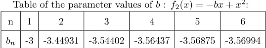
We remark the emergence of a decreasing sequence of the parameter values of b : {b1;b2;b3, ...}which
correspond to flip bifurcation values. These values ofbtend towardsb1such the attractor becomes a Cantor
set.
Table of the parameter values ofb: f2(x) =−bx+x2:
n 1 2 3 4 5 6
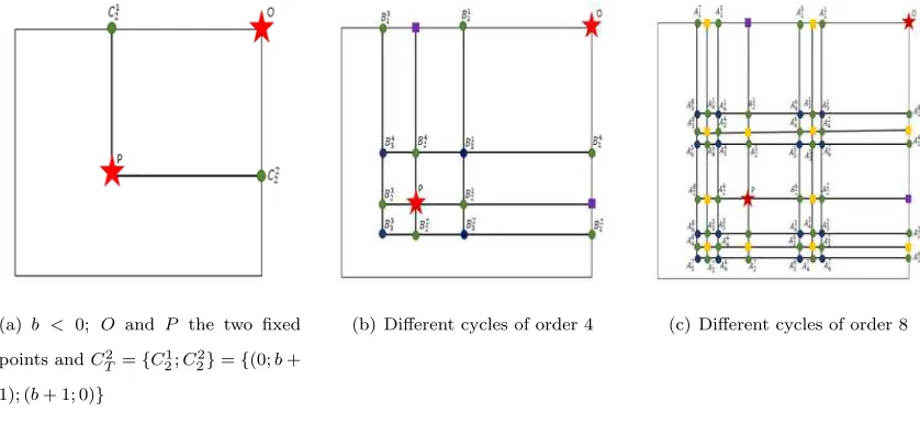
We give the position of cycles for the map T and precisely cycles which are generated by an infinite
sequence of flip bifurcations and provocate chaos. The two fixed pointsOandP can be stable inside a given
region of the space of the parameters of the map, and can lose stability via a Hopf bifurcation, as well as a
transcritical bifurcation or a flip bifurcation. This last situation is reported in the qualitative Fig. 2.(a, b, c)
forb <0, whenO is unstable andP a stable point.
(a) b < 0; O and P the two fixed points andC2
T={C21;C22}={(0;b+
1); (b+ 1; 0)}
(b) Different cycles of order 4 (c) Different cycles of order 8
Figure 2. Different cycles forb <0.
Other pecular properties that can be deduced from the properties of the one-dimensional map f2(x) for
the endomorphismT whena= 0 concern critical curvesLC−1,LC,LC1,LC2which are given here by
LC−1: x=s−1; wheres−1=b2 is the critical point of rank 0 off2(x)
and
LC: y=s0=f2(s−1);LC1: x=s0=−b
2
4
LC2: y =s1;LC3: x=s1
withsk =f2(sk−1) of rank (k+ 1)
For b = −2, the critical points s−1, s0, s1 are equal, b < −2, the interval I = [s0, s1] is an absorbing
interval containing an attracting set, but forb >−2, the intervalI= [s0, s1] is not an absorbing interval.
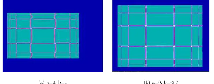
For selected values of the parameter b and forn= 2, the coexistence of many different local attractors
opens an important question on their behavior, and the problem of the delimitation of the boundaries of their
basins which are made up of rectangles. In Figures 3.(a, b), the immediate basin (containing attractors) is
formed by disjoint rectangles bounded by segment of the critical curves which are straight lines parallel to the
coordinates axes, and issued from the critical points off2(x). Studying these basins help in understanding
the ways of multistability formation. We refer to [13] for its complete description.
The bifurcation curves related to the two values ofb= 1 andb=−3.7 correspond to homoclinic bifurcation
curves for the fixed pointsO orP and determine also the end of the range in which the quadratic shape of
(a) a=0; b=1 (b) a=0; b=-3.7
Figure 3. Basins and critical curves.
4. Basins and invariant curves
We present some results of numerical simulations and discuss their implications. We have to explain the
creation of two invariant curves, one issued from a fixed point of saddle type, constitutes the basin boundary
of the second one which is an attracting closed curve. The phase portrait of the quadratic endomorphism
T is studied by constructing regular invariant curves associated to saddles and Hopf bifurcation. In this
section, the regions of parameters chosen for numerical experiments contain parametric values which are not
arbitrary but characteristic values with focus on selected properties. Thus, in the following we shall focus
our attention on the description of the bifurcations which are expected to occur as we vary the parameters
aclose to 2 in (a) and (b) and −2 in (c) and (d) andb close to the value 1. Sinceb >0, the fixed pointO
is stable, inside its attraction basin undergoes a Hopf bifurcation and a little closed curve exists inside the
basin, together with a closed stable manifoldof the saddle pointP.
The following figures show the corresponding basin structure of T for n = 2. Figures 4.(a, b, c, d, e, f)
represent the existing attractors (the two fixed points O;P, an invariant closed curve (ICC) around the
fixed pointO after a Hopf bifurcation) and the stable manifold emanating from the saddle point. In Figs
4.(a, b)a '2, b'1 (λ1= λ2= 1),the two fixed points exist,P is a saddle and its invariant stable manifold
delimits the basin ofO which has undergone a Hopf bifurcation whenauncreases from 1.7 to 1.9. The two
curves are closed and invariant. In Figs 4.(c, d),a ' −2, b= 1 (λ1= λ2=−1), the fixed pointOundergoes
the flip bifurcation Λ1 (1 +b+a= 0) and the 2−cycle is still merged withO which gives again a ICC. In
Figs 4.(e, f), and forn= 4 we have nearly the same behavior with invariant curves associated with the fixed
points. We observe that small changes in the location of the critical curve LC−1 which has some effects
on the properties of the attractors, and it may cause remarkable asymmetries in the structure of the basins,
(a) Invariant closed curve in a yel-low basin n=2
(b) Only invariant curves are displayed n= 2, x={−0.36, ..,1},
y={−0.28, ..,0.15}
(c) Invariant closed curve in a yellow basin n=4
(d) Only invariant curves are displayed n= 4, x={−1, ..,1},
y={−0.28, ..,1}
(e)a >0 (f)a <0
Figure 4. Bounded basin delimited by the invariant stable manifold and an ICC around
the stable fixed point.
Other invariant sets forn= 2 (and similarly forneven) can be estimated forT2. These invariant sets are
obtained by iterating invariant lines in the immediate bounded basin. The casea=−2 is very interesting,
because we can put in evidence the existence of such sets. The special character of this kind of sets has been
already observed in uncoupled maps. To illustrate the idea, we put L1: y2 =αx2+β, x2 andy2 are the
second iterates ofxandy. We obtain then a(ay−bx+x2)−by+y2=α(ay−bx+x2) +β. By virtue of
invariance ofL1byT (y=αx+β),we have :
For allx,(a+α2−α)x2+ (a2α−ab+ 2αβ−aα2)x+ (a2β−bβ+β2−aαβ−β) = 0.
Then a+α2−α= 0 ; β(−b+β−aα2−1) = 0 and−ab+ 2αβ−aα3= 0
Fora=−2, we haveL1:y=−x+b−1.If we takeb= 1 +ε,thenL1:y=−x+ε
The iteratesT(L1) are also invariant becauseT2(T(L1)) =T(T2(L1)) =T(L1).
T(L1) is a parabola whose equation is y= x
2
α2 + (a−
b α−
2β α2)x+
β α
If we takeβ = 0,we have L2:y= 0, L3:y=x.
Besides the elements seen thus far, there is another particularity in the dynamics of T. The strong
dependence on the parameters causes a rich variety of complex patterns on the plane and gives rise to
different kinds of basins. Taking into account the complexity of the matter and its nature, the study of these
phenomena can be carried out only via the association of numerical investigations guided by fundamental
considerations that can be found in [13]. The endomorphism (2) with a 6= 0 is of type (Z0−Z2), whose
three first critical curvesLC−1,LC,LC 0
1are given here by
LC−1:
(x, y)/x= b2
and
LC: T(LC−1) =
n
(x, y)/y=ax−b2
4
o
LC1:
n
(x, y)/y= 1
a2x
2+ (a+ b2
2a2 −
b a)x+
b4
16a2 −
b3
4a
o
The inversesT±−1 are given by:
T±−1(x, y) =
x= b2±1 2
p
b2+ 4(y−ax)
y=x
(8)
Attractors constitute an interesting set of study by themselves. Their attraction basins are split in two equal
parts byLC−1.
To understand the behavior of the map when ais close to −2, we follow the evolution in the phase plane
when we vary the parameterb (b≈ −5.87,b= 0.95).
All these situations have been shown in [13] proposed by Mira et al. for a wide variety of reasons and different
models, in all they incorporate nonlinear terms and quadratic nonlinearities. In most cases, the basin of
attraction undergoes some changes. The geometric structure of the basin is occurring for particular choices
of the parameters.
Recent works dealing with cases of multiple attractors in noninvertible maps have highlighted how
nonin-vertibility can become a source of bifurcations and complex structure in the basins of attraction. However,
the global phenomena and the complex structures of the basins shown here are due to the both sets which
are critical and invariant sets.
Fora=−2, the critical curvesLC−1,LC,LC1andLC2delimit the attractor that occupies the whole basin.
The invariant lines of T and T2 respectively (y =x andy =−x+ 1) contain fixed points (0,0) and (5,5)
fory=xand the two points of the 2−cycle{(2,−1); (−1,2)}fory=−x+ 1 (see Fig. 6.).
5. Conclusion
This family of polynomial maps withn= 2 is symmetric with respect to the curveLC−1. And the bifurcations
shown in the different sections are related to this curve, but we can observe that basins become asymmetric
(a) Connected basin (b) Bifurcation basin to non-connected basin
(c) Nonconnected basin,b < 0
(d) Nonconnected basin,b > 0
Figure 5. The evolution of basin in the phase plane.
Figure 6. Critical and invariant sets fora=−2.
global bifurcations. According to the bifurcation diagram shown in Fig.1(a) and by exploiting the relation
between invariant sets and critical curves, we have considered four Parametric points (a, b) which are of
two or three codimension bifurcation points, (−2,1), (−2,−7), (2,1) and (0,−1). The two first points are
of two-degree of complexity and the two last points are of three-degree of complexity, the behavior of the
solutions is mainly determined by the invariant sets and critical curves. We are not trying to show the
details of the bifurcation mechanisms leading to the dynamic situations described above for n= 2k, k >1,
however, we believe that they have identical behavior to those observed in Secs. 2 and 3, and display the
same structure associated with the basin bifurcation connected-nonconnected described in Sec. 4, even if
they occur in a very narrow interval of values of the parameterb.
References
[1] G. S. Agarwal, Existence of multistability in systems with complex order parameters, Phys. Rev. A, 26 (1982), 888–891. [2] F. T. Arecchi, R. Meucci, G. Puccioni and and J. Tredicce, Experimental evidence of subharmonic bifurcations,
multista-bility, and turbulence in a q-switched gas laser, Phys. Rev. Lett., 49 (1982), 1217–1220.
[3] R. L. Clerc and C. Hartmann, Invariant manifolds of separable discrete dynamic systems, Dynamics Days, La Jolla, California, (1982).
[5] M. R. Ferchichi, I. Djellit and J. C. Sprott, Broken symmetry in modified Lorenz model, Int. J. Dyn. Syst. Differential Equations, 5 (2) (2015), 136-148.
[6] U. Feudel and C. Grebogi, Multistability and the control of complexity, Chaos, 7 (1997), 597–604.
[7] C. Grebogi, E. Kostelich, E. Ott and J. A. Yorke, Multi-dimensioned intertwined basin boundaries: Basin structure of the kicked double rotor, Physica D, 25 (1987), 347–360.
[8] I. Gumowski, C. Mira, Dynamique chaotique, Ed. Cepadues, Toulouse, (1980).
[9] M. Henon, A two-dimensional mapping with a strange attractor, Commun. Math. Phys., 50, (1976), 69–77.
[10] K. Ikeda, Multiple-valued stationary state and its instability of the transmitted light by a ring cavity system, Opt. Commun., 30 (1976), 257–261.
[11] H. W. Lorenz, Multiple attractors, complex basin boundaries, and transient motion in deterministic economic systems, in Dynamic Economic Models and Optimal Control, ed. Feichtinger, G. (Elsevier), (1992).
[12] C. Mira, Chaotic dynamics, World Scientific, (1987).
[13] C. Mira, L. Gardini, A. Barugola and J. C. Cathala, Chaotic dynamics in two-dimensional non invertible maps, World Scientific, (1996).
[14] B. Razafimandimby, Domaine d’influence de certaines singularit´es stables d’un endomophisme deR2, Th`ese de 3`eme cycle,