This is a repository copy of
Partition-based algorithm for estimating transportation network
reliability with dependent link failures.
.
White Rose Research Online URL for this paper:
http://eprints.whiterose.ac.uk/84670/
Version: Accepted Version
Article:
Sumalee, A and Watling, DP orcid.org/0000-0002-6193-9121 (2008) Partition-based
algorithm for estimating transportation network reliability with dependent link failures.
Journal of Advanced Transportation, 42 (3). pp. 213-238. ISSN 0197-6729
https://doi.org/10.1002/atr.5670420303
[email protected] https://eprints.whiterose.ac.uk/
Reuse
Unless indicated otherwise, fulltext items are protected by copyright with all rights reserved. The copyright exception in section 29 of the Copyright, Designs and Patents Act 1988 allows the making of a single copy solely for the purpose of non-commercial research or private study within the limits of fair dealing. The publisher or other rights-holder may allow further reproduction and re-use of this version - refer to the White Rose Research Online record for this item. Where records identify the publisher as the copyright holder, users can verify any specific terms of use on the publisher’s website.
Takedown
If you consider content in White Rose Research Online to be in breach of UK law, please notify us by
Partition-based Algorithm for Estimating Transportation Network Reliability with
Dependent Link Failures
Agachai Sumalee1* David P. Watling2
1
Department of Civil and Structural Engineering, The Hong Kong Polytechnic University
2
Institute for Transport Studies, University of Leeds
Abstract
Evaluating the reliability of a transportation network often involves an intensive simulation exercise to randomly generate and evaluate different possible network states. This paper proposes an algorithm to approximate the network reliability which minimizes the use of such simulation procedure. The algorithm will dissect and classify the network states into reliable, unreliable, and un-determined partitions. By postulating the monotone property of the reliability function, each reliable and/or unreliable state can be used to determine a number of other reliable and/or unreliable states without evaluating all of them with an equilibrium assignment procedure. The paper also proposes the cause-based failure framework for representing dependent link degradation probabilities. The algorithm and framework proposed are tested with a medium size test network to illustrate the performance of the algorithm.
1. Introduction
In system engineering, reliability may be defined as the degree of stability of the quality of service that a system normally offers (Bell and Iida 1997). In a transport system, such as a road network, there are two key elements contributing to the level of service: the travel demand and the system supply. The degree of stability of a transport network can be interpreted as the ability of the network to meet expected goals measured by some indicators under different circumstances (e.g. variability in flows and physical network capacities). A range of different indicators have been proposed to measure this
*Corresponding author’s email:
degree of stability, depending on the features of variability modeled and the objectives of the analysis. These indicators include connectivity reliability (Asakura et al. 2003), network vulnerability (Berdica 2002; Taylor et al. 2006), capacity reliability (Chen et al. 2002; Sumalee and Kurauchi 2006), travel time reliability (Asakura 1999; Du and Nicholson 1997), total travel time reliability (Clark and Watling 2005; Sumalee et al. 2007), and demand satisfaction (Heydecker et al. 2007). In the present paper, we shall specifically focus on problems in which link capacities are variable (stochastic), and where the aim is to compute a travel time reliability index.
The initial impetus for research in the area of stochastic capacity reliability analysis arose from the study of major natural events, such as earthquakes, affecting the ‘connectivity’ of the network (Bell and Iida 1997). Each link is assumed to have an independent, probabilistic, binary mode of operation (Wakabayashi and Iida 1992); at one extreme, the link states might represent whether the link is
‘open’ or ‘closed’, though they could represent other interpretations of the successful operation of a link. The objective of connectivity reliability analysis is then to compute the probability that an origin-destination movement will be connected by at least one path consisting of all ‘open’ links, though without regard to how efficient that path may be or whether travellers may choose to use it.
Travel time reliability analysis extends the concept of connectivity analysis in several ways. Firstly, more generally, we view the impacts of unreliability through the change of the ‘mode’ of each link, where a link is assumed to have multiple modes of operation (Du and Nicholson 1997). Specifically, in the context of capacity variability, the modes of each link may represent alternative, discrete reductions in link capacity, which can be caused by some natural or man-made incidents. (Alternatively we may consider a continuous distribution of link capacity, see (Lo and Tung 2003), though in this paper we shall adopt a discrete representation).. Secondly, for any given ‘network
is concerned with the probability of any path being available, however long the travel time, travel time reliability is concerned with the probability of availability of a path with an acceptable travel time.
We make two observations about the class of problem described above, which together motivate our work. Firstly, aside from whether the link mode is assumed to be binary, multi-mode or continuous, a common theme to the approaches cited above is the assumption of statistical independence between links in the degradation model. An exception may be found in an extension by Chen et al (2002) to their basic model, with capacities assumed to be correlated across links. While the independent link failure assumption may be justified in some domains, it may be implausible for the study of transport networks since the degradation of different links may often have common underlying causes (e.g. flood, snowfall or earthquake). In such cases, assuming independence will tend to provide an over-optimistic estimate of performance, since the common causes are likely to simultaneously affect a number of alternative routes. On the other hand, the assumption of dependent link failure probabilities may impose more complexities on the problem and hence require more computational time to evaluate the network reliability performance. The paper proposes the cause-based framework (as described in the next Section) in which different causes of failures are defined (e.g. flood or earthquake). Under each cause, the independent link degradation probabilities can be defined separately. Despite the independence of link degradation under each cause of failure (so-called conditional independence), the causal tree structure gives rise to an implicit specification of correlated (dependent) link degradations.
The second observation we make is that computation of the reliability measure is also a major challenge, especially if realistic correlation and user-behavior models are to be adopted. Even if we were to make the simplifying (unrealistic) assumption of independent link failures and binary operate/fail states, for example, with 50 links the number of combinations is substantially larger than 1014, and so we cannot hope to solve the problem by enumeration of all possible states, since each typically requires the solution of an equilibrium problem1 To tackle this issue, early developments have adopted Monte Carlo simulation (MC) to generate supply and/or demand uncertainties for the
1
equilibrium-based traffic model. Du and Nicholson (1997) simulated the network capacity degradation level using MC to establish the lower and upper bounds of the network reliability indicator. Similarly, Chen et al (2002) and Sumalee and Kurauchi (2006) adopted MC to evaluate network capacity reliability. The flexibility of MC comes with the trade-off of a potentially high computational burden.
Based on these observations, and the appeal of using MC for representing conditional independence, Sumalee and Watling (2003) proposed a method for estimating travel time reliability under dependent link failures, which operates by identifying those network states with large probabilities in order to reduce the total number of considered network states. However, this approach will be efficient only if some scenarios have high probabilities (and others are trivial states). The present paper proposes a different approach to avoid this pitfall by dissecting the network states into a number of reliable, unreliable, and un-determined partitions. The paper postulates an important monotone property of the reliability function, which will be clarified later in Section 3.2. This assumption will allow us to determine a number of reliable and unreliable partitions by evaluating only a few network states with a network assignment model. Some undefined partitions will remain after applying this algorithm in which the stratified MC (as described in Section 3.4) will be applied to evaluate their associated reliability probabilities.
2. Notation and preliminaries
2.1 Stochastic network definition under cause-based failures
different causes.
Under the cause-tree, there are several possible scenarios with different combinations of the active causes. Let Sw=
(
Rw1,K,Rwm,KRwM)
denote a realized scenario where w and m is the index of thescenario and cause respectively. m w
R denotes the status of cause m as realized in scenario w in
whichR = if cause m occurs in scenario w and wm 1 0
m w
R = otherwise. Let Pm be the probability of
cause m to occur. The probability of scenario w can be defined as Pr
( )
( )
mw w
m
S e
"
=
Õ
, wherem
w Pm
e = if m 1
w
R = and m 1
w Pm
[image:6.595.76.523.310.523.2]e = - otherwise.
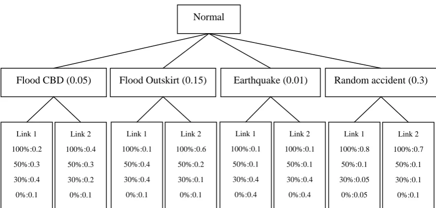
Figure 1: Example of the cause-based failure probability tree As shown in Figure 1, under each cause m the link is associated with a probability, ,
e j m
P , for the link j
to be in mode e, where e, j m
C denotes the % of capacity disruption of the link under this mode.
Within each scenario many causes may occur simultaneously. Thus, the link may be degraded by different causes. Under each scenario, different combinations of the realized link degradation level are possible. We denote each realized combination of the link degradation levels as
( )
{
1}
,1, , , , , ,
m M
e
e e
w
j t Cj Cj m Cj M
f º % K % K % where t is the index of a possible combination and e% is the realized m
disruption level of link j under cause m in this combination. Note that if m 0
w
R = , then e,m 100
j m
C% = . Normal
Flood CBD (0.05)
Link 1 100%:0.2 50%:0.3 30%:0.4 0%:0.1 Link 2 100%:0.4 50%:0.3 30%:0.2 0%:0.1 Link 1 100%:0.1 50%:0.4 30%:0.4 0%:0.1 Link 2 100%:0.6 50%:0.2 30%:0.1 0%:0.1 Link 1 100%:0.1 50%:0.1 30%:0.4 0%:0.4 Link 2 100%:0.1 50%:0.1 30%:0.4 0%:0.4 Link 1 100%:0.8 50%:0.1 30%:0.05 0%:0.05 Link 2 100%:0.7 50%:0.1 30%:0.1 0%:0.1
The aggregate degradation level on a link under the realized state w
( )
j t
f is assumed to follow:
( )
(
)
( ) , , , mem w j m j
e w
j w j j j m
C t
C t C C
f f " Î æ ö÷ ç ÷ ç
= ×ç ÷÷÷
çè %
Õ
ø%
(1)
where C is the normal capacity of link j. For instance, suppose that the original capacity of link j is j
1,000 PCU/hr and there are two active causes which degrade the link capacity to 750 (75%) and 800 (80%) PCU/hr respectively. The accumulated effects of these two causes on this link will result in the link taking the degraded capacity of 1000 0.75 0.80´ ´ = 600PCU/hr. We remark that for each cause the number of possible degraded link capacities is defined a priori. However, due to the effect of different causes on the same link, a number of different degraded link capacities will be created. The probability of link j to take each mode can be defined as:
( )
(
)
(
)
( )
( ) , , ,Pr Pr m
em w j m j
e w
j w j w j m
P t
C t S P
c f " Î =
Õ
% % (2), where
( )
{
1}
,1, , , , , ,
m M
e
e e
w
j t Pj Pj m Pj M
c º % % %
K K . Different ,
(
( )
)
w
j w j
C f t under different w
( )
j t
f may have the
same value. Thus, ,
(
( )
)
w
j w j
C f t can be grouped into a number of possible link mode for each link.
For each link j, let 1
, l, , L
j j j
C KC K C be a set of possible link capacities (modes). For each l j
C , we can
define the total probability of the link to take this mode as:
( )
(
)
(
)
, Pr ,
l t w
j j w j w j
w t
p u C f t
" "
=
å å
× (3)where , 1 t j w
u = if ,
(
( )
)
w l
j w j j
C f t = C , and , 0 t j w
u = otherwise.
Let
(
1)
1, , , ,
J l l
k C k CJ k
k = K be a possible network state k in which lj is the mode (or finite capacity) of link
j realized in this state, where ,
{
1, , ,}
jl l L
j k j j j
C Î C KC K C . For brevity, we will define the network state
k as
(
1k, , k)
k l lJ
k = K which is the vector of the realized link modes in this network state. Also let
k k
k
"
W=
U
be the set of all possible network states. The probability of the state can then be defined as:( )
Pr k j l k j j p k "=
Õ
(4), where k j
l is the realized mode of link j in the network state k and lkj j
2.2 Partial user equilibrium route choice condition
Under the normal circumstance, the notion of Wardrop’s user equilibrium (UE) has been extensively used to describe how travelers choose their routes in the network. However, the behaviors of travelers under degraded conditions of the network may be different. Under severe events such as natural disasters, the driver’s main objective is likely to be his/her safety. The routing may also be controlled by a ‘network regulator’, perhaps according to a predefined strategy (Sumalee and Kurauchi 2006). In less severe or post-disaster cases, it might be expected that the drivers will partially adapt their travel choices (such as route/mode choices) responding to the degraded network conditions. In this paper, the concept of partially adaptive behavior of travelers is assumed which is defined as follows.
Let W be a set of origin-destination pairs in the network in which P is the set of paths connecting rs
origin r to destination s. Under the un-degraded network condition, the UE assignment is used to determine the normal flows in the network. Let UE
p
F be the path flow solution of UE assignment at
the normal network state. Note that the problem of non-uniqueness of the UE path flows can be dealt with by selecting the most-likely path flow (Larsson et al. 1993) or adopting the stochastic user equilibrium model instead. Under the degraded network statek , the travel time of each link, k
(
, ,)
l
j j j k
t v C , is a function of the realized link mode (capacity) and the link flow. A set of affected
paths can then be defined, namely those paths that contain at least one degraded link. Let P% denote rs
the set of affected paths between an O-D pair (rs) under scenariok . Under the partially adaptive k
behavior assumption, only those drivers on the affected paths, F% forq qÎ P% , will consider rerouting. rs
On the other hand, those drivers on the unaffected paths pÎ P - Prs % will remain on the same routes rs
followed in the un-degraded network..
, 1
, 1
, 0
0, , 0
j
l
q jq j k jk p jp j k rs
j k p
j
l
q jq j k jk p jp j k rs
j k p
F t F F C
q
F t F F C
d d d m
d d d m
=
=
æ æ ææ ö öö ö÷
ç ç çç ÷ ÷÷÷ ÷
ç ç ÷ ÷
×èççç çèç × çèççççèç × + × ø÷÷ ÷÷÷ø÷÷÷ø- ÷÷÷÷ø=
"
æ æ ææ ö öö ö÷
ç ç çç ÷ ÷÷÷ ÷
ç ç ÷ ÷
³ èççç çèç × çèççççèç × + × ø÷÷ ÷÷÷ø÷÷÷ø- ÷÷÷÷ø³
å
å
å
å
å
å
%
%
(
)
,kÎ P " Î P - P "%rs; p rs %rs; r s, Î W(5)
, where m is the minimum travel cost for the OD pair rs and rs d =jq 1if link j is related to path q and
0
jq
d = otherwise. Under the symmetric condition of the link cost Jacobian (or assume a typical
separable link cost function), the problem can be reformulated as a minimization problem:
(
)
ˆ , ˆ 0 , , min , . . ˆ ; 0 ;j
rs rs rs
rs rs
v
l
j j k
j
j q jq p jp
q rs W p rs W
q q rs q q rs
q q
q rs
t x C dx s t
v F F j A
F F rs W
F q rs W
d d
Î P " Î Î P - P " Î
Î P Î P
= × + × " Î
×D = ×D " Î
³ " Î P " Î
å ò
å
å
å
å
v % % % % % % (6)where v is the link flow and ˆj Dq rs, = if path q is related to OD pair rs and 0 otherwise. The 1
existence and uniqueness of the solution to this optimization problem follows the original problem of the UE assignment. Note that the algorithm proposed in this paper can also be applied to other modeling frameworks (e.g. SUE or even micro-simulation).
2.3 Reliability performance function and its monotonicity postulation
As reviewed, various indicators have been proposed in the literature; each of which is appropriate for different circumstances. In this paper, the focus is mainly on the performance of the network after a major disruption in coping with recovering travel demands. During the post-disaster period, the activities and travel patterns in an urban area are gradually resume to the normal condition (Sumalee and Kurauchi 2006). Thus, the key performance requirement adopted is based on the travel time reliability principle in which the network is considered reliable if after the degradation the travel times of all used paths in the network are under some given thresholds.
Let r denote the travel cost of path p under network state p k , i.e. k
( )
(
ˆ, ,)
lp k j j j k jp
j A
t v C
r k d
" Î
=
å
and( )
k( )
1p kk
¡ = if rp
( )
kk £ np×rp( )
k0 and ¡ p( )
kk = 0 otherwise. Note that k and 0 rp( )
k0 are thenormal network state (no degradation) and the associated path travel time of path p under the normal state. Note that for the unused path under the normal condition we assume rp
( )
k0 to be equal tothe minimum OD travel time. Let np³ 1 be the tolerance factor for the path travel time. The
reliability function of the network can then be defined as:
( )
k 1 p( )
k 1p
f k iff k
"
=
Õ
¡ = and( )
k 0f k = otherwise. The network reliability can be defined as the probability that the network will
function:
( )
(
)
(
( ) ( )
)
Pr k 1 Pr k k
k
f k k f k
"
Z = = =
å
× (7)In this paper the reliability performance function is assumed to be a monotone non-decreasing function. For any two network states, k and k k , the monotone property of the reliability function implies that: v
( )
{
1 and}
{
, ,}
( )
1j j
l l
k j k j v v
f k = C £ C " Þj f k = (8)
( )
{
}
{
1 1}
( )
, ,
0 and l l 0
k j k j v v
f k = C ³ C " Þj f k = (9)
Noteworthy, this postulation of the monotone reliability function should be sensible and applicable to most cases except the network with the potential Braess paradox effect. Nevertheless, our main justification for this postulation is twofold.
First, we can establish a proof for the monotonicity of the reliability function in (7) by assuming that there exists at least one unaffected path for each OD pair. Under the normal condition, the path travel costs on all used routes are equal due to the UE condition. Due to the definition of the partial UE, only those flows on affected routes will reroute. Thus, the travel cost on the unaffected route can only increase due to the monotone property of link cost functions, whereas the travel time on this unaffected route will form a bound for the new travel time on all affected routes. The second justification is that our algorithm will always be pessimistic in terms of reliability, since it ignores the Brasses paradox effect that reducing capacity can improve reliability. This pessimistic estimation should be consistent with the objective of evaluating the network against the worst-case scenario.
This section proposes a method for efficiently evaluating the upper and lower bounds of the network reliability function as defined in (7). The evaluation of the reliability function in (7) can be viewed as a process of identifying all possible network states k
k
k
"
W=
U
and then evaluating each state in turn bysolving (6) to identify the set of reliable network states, denoted by R
{
where( )
1}
k k f k
k k
W = " =
(also denote W as the set of unreliable states). Instead of exhaustively evaluating all possible states, U different subsets of W containing several network states will be defined and each subset evaluated as to whether it is reliable (all states in the subset are reliable), unreliable (all states in the subset are unreliable) or undetermined. Then, the algorithm will find a different way to dissect the remaining undetermined subsets so that the newly defined subsets can be categorized as either reliable or unreliable. The subsets of Wwill be termed partitions as defined in the next section.
3.1 Definition of the partition of network states
A partition s is a subset of W which contains network states,
(
1, ,)
k k
k l lJ
k º K , in which
s k s
j lj j
a £ £ b for all links. Let s 1s, , s J
a = éëa K a ùû and s 1s, , s J
b = éëb K b ùû. Thus, the partition s is
denoted as s, s
a b
é ù
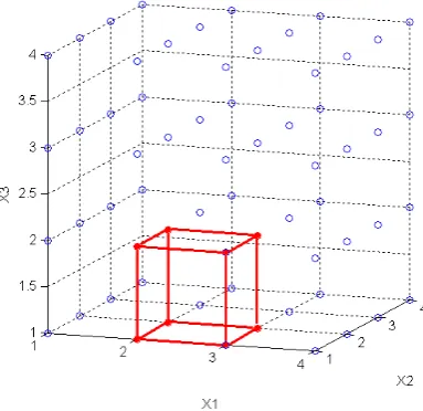
ë û. Figure 2 illustrates an example of a three-dimensional state space of W where all links have four possible link modes (capacities). The cube in the figure indicates the states that constitute the partition s, s
a b
é ù
ë ûwhere s
[
2,1,1]
a = and s
[
3, 2, 2]
b = . Based on (2) and (3), the
probability of s, s
a b
é ù
ë ûcan be defined as:
(
)
(
)
Pr , Pr
s j
s j
s s s s l
j j j j
j j l
l p
b
a
a b a b
" " =
ì ü
ï ï
ï ï
é ù = £ £ = í ý
ë û ïï ïï
î
å
þÕ
Õ
(10)where plj is as defined in (3). We denote the reliable, unreliable, and undetermined partition as
, R
s s
a b
é ù
ë û, s, sU
a b
é ù
ë û , and s, s D
a b
é ù
ë û respectively. Note that R s, s R s
a b
"
é ù
W =
U
ë û , U s, s U sa b
"
é ù
W =
U
ë û , and, D
D s s
s
a b
"
é ù
W =
U
ë û . Clearly, W= W È W È WR U D. Thus, we can also redefine (7) as:
( )
( )
( )
( )
When all the undetermined partitions are assumed to be unreliable, we obtain the lower bound of the reliability function (i.e. Pr
( )
RZ
W £ ). On the other hand, if all the undetermined partitions are
assumed to be reliable, the upper bound of the reliability function can be formed (i.e.
( )
( )
( )
1 Pr U Pr R Pr D
Z£ - W = W + W ). The gap between the lower and upper bounds is, thus, exactly
( )
Pr D
W . The algorithm proposed indeed aims to minimize this gap by dissecting those
[image:12.595.212.404.252.438.2]undetermined partitions to either reliable or unreliable partitions.
Figure 2: Example of a partition in three link network
3.2 Partition algorithm
Initially, the set of all network states will be defined as an undetermined partition, i.e. D
W = W. Then, the partition algorithm based on Doulliez and Jamoulle (1972) can be adopted to sequentially define different reliable and unreliable partitions to minimize the size of the total probability space of
D
W . The algorithm will utilize the monotone property of the reliability function as postulated in Section 2.3. Two indices of the link mode employed to dissect the undetermined partition are all-links reliable cut-off index and single-link reliable cut-off index. For each undetermined partition,
, D
s s
a b
é ù
ë û, the all-link reliable cut-off index, denoted by q ,can be defined as: s
( )
(
)
{
1}
min 0 where s , , s
s f k k J
q = q k = k º b - qK b - q (12)
, where s j
b - qindicates the mode number of the capacity of link j, i.e. , sj
j k j
C = Cb-q. q is the s
state to be evaluated as unreliable. In practice, this can be found by setting all link modes at s j
b and
then gradually decreasing all link modes with a discrete step of q =1, 2,3,K until the network state becomes unreliable. This all-links reliable cut-off index can be used to determine the feasible and infeasible partitions following (8) and (9):
1, and ,
s s R s s U
s s
b q b a b q
é - + ùÎ W é - ùÎ W
ë û ë û (13)
The single-link reliable cut-off index, denoted by s j
l , can determine addition unreliable partitions.
s j
l is defined for each link in turn for each undetermined partition:
(
)
{
1}
min , , , 0
s s s s
j f j J
l = l b K b - l b = (14)
Note that l sj³ qs due to the monotone property of the reliability function. For a given éëas,bsûùDand
s j
l , an unreliable partition can be defined as:
, where and
s v U v s s v s
j j j i i i j A
a b b b l b b
é ùÎ W = - = " ¹ Î
ë û (15)
The unreliable partition as defined by q , s s, s U s
a b q
é - ùÎ W
ë û , may overlap with the additional
unreliable partitions defined by l causing problems for the calculation of sj Pr
( )
UW . Thus, a
disjoint unreliable partition can instead be defined for each s j
l and q as: s
and
, where = and 1
= and
v s v s
i i s i i
v v U v s v s s
i j i j j
v s v s
i j i j
i j i j i j
a b q b b
a b a a b b l
a a b b
ì ü
ï = - = < ï
ï ï
ï ï
ï ï
ï ï
é ùÎ W í = - - = ý
ë û ïï ïï
ï = > ï
ï ï
ï ï
î þ
(16)
For a given s, s D
a b
é ù
ë û , after excluding the reliable and unreliable partitions as defined in (13) and (16),
the remaining undetermined partitions can be defined for each s j
l and q as: s
and
, where = and 1
= and
v s v s
i i s i i
v v D v s s v s
i j j i j s
v s s v s
i j j i j
i j i j i j
a b q b b
a b a b l b b q
a b l b b
ì ü
ï = - = < ï
ï ï
ï ï
ï ï
ï ï
é ùÎ W í - = - - = ý
ë û ïï ïï
ï - = > ï
ï ï
ï ï
î þ
(17)
the input maximum number of iterations of the partition algorithm and J is the number of links in the network.
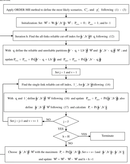
Figure 3: Overall procedure of the partition algorithm
In the first stage of the algorithm, the ORDER-MII method as adopted by Sumalee and Watling (2003) will be applied to sort the scenarios by their probabilities to choose the set of most probable scenarios.
Initialization: Set D
W = W; s, s D
a b
é ù= W
ë û ; Plower= 0; Pupper =1; and h= 1
Iteration h: Find the all-links reliable cut-off index for s, s s
a b q
é ù®
ë û following (12)
Find the single-link reliable cut-off index, s j
l , for s, s
a b
é ù
ë ûfollowing (14) Set j = 1 and v = 1
j = J With qsand s
j
l define v, v U
a b
é ùÎ W
ë û following (16) and update Pr
(
v, v)
upper upperP = P + éëa b ùû; also
define v, v D
a b
é ùÎ W
ë û following (17) and calculate Pr v, v v
P = éëa b ùû With qsdefine the reliable and unreliable partitions 1,
s s R
s
b q b
é - + ùÎ W
ë û and s, s U
s
a b q
é - ùÎ W
ë û ; and
update Pr
(
s 1, s)
lower lower s
P = P + ëéb - q + b ùû and Pr
(
s, s)
upper upper s
P = P + éëa b - qùû
Set j = j+1 and v = v+ 1 NO
Choose v, v D
a b
é ùÎ W
ë û with the maximum Pr
(
v, v)
vP = éëa b ùû; Set s = s+ 1and s, s v, v
a b a b
é ù é= ù
ë û ë û
and update D D R U
W = W - W - Wand h = h +1 h = H
NO YES
Terminate YES
Apply ORDER-MII method to define the most likely scenarios, C , and lj l j
Then, the set of link capacities (modes) can be determined using the product operator as defined in (1), and the probability of each link mode can be calculated following (2) and (3).
3.3 Application of the stratified Monte-Carlo simulation to undetermined partitions
After reaching the maximum number of iterations of the partition algorithm, a number of undetermined partitions will still remain (as shown in Figure 3) in which the gap between upper and lower bounds of the reliability function will be equal to Pr
( )
DW . The quality of the estimation of
the reliability index is relative to this gap. A strategy to further improve the quality of the estimation is to apply Monte-Carlo simulation (MC) to evaluate these remaining undetermined partitions. In this section, an improved sampling strategy will be incorporated with MC.
From the set of undetermined partitions (let V be the total number of remaining undetermined partitions), each partition is associated with its total probability, i.e. Pr
(
v, v)
v
P = éëa b ùû. This
probability signifies the importance of this partition in improving the estimation. For a given total sample size N, different sample sizes will be allocated to different partitions depending on their probabilities, i.e.
(
)
(
)
1
Pr , Pr ,
v v
v V
v v
v
n N a b
a b
=
é ù
ë û
=
é ù
ë û
å
(18)where nv is the number of samples (draws) to be obtained from partition v. This is the so called
stratified sampling method. Then, for each partition MC will draw different network states (up to nv
samples) and evaluate them in turn. Let O denote the total number of reliable states from the v
samples of partition v. We can then update the upper and lower bound as:
(
)
Pr v, v v
lower lower
v
O
P P
n a b
é ù
= - ë û (19)
(
)
Pr v, v v v
upper upper
v
n O
P P
n
a b
-é ù
= - ë û (20)
4.1 Test descriptions
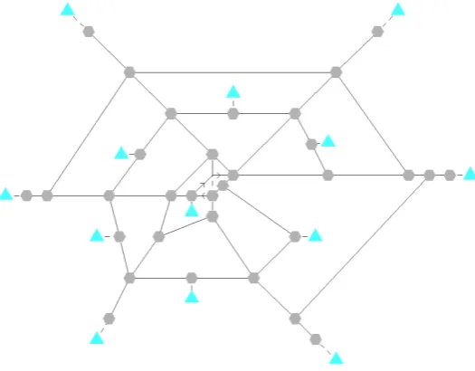
[image:16.595.163.426.153.358.2]The test network as displayed in Figure 4 has 89 directed links with 14 zones and 182 O-D pairs (neglecting intra-zonal movement) where triangle nodes represent zones.
Figure 4: Test network for the partition algorithm
The tests involve evaluating the reliability measure as defined in (7) with three different demand levels including the base demand, 1.5
base demand, and 2
base demand, and with six different tolerance factors (n ) for travel time, i.e. 1.5, 2, 2.5, 3, 3.5, and 4. Following the cause-based structure as pdiscussed in Section 2.1, ten possible causes of failure are assumed (see Table 1).
Cause Probability of cause not to occur Probability of cause to occur
1 0.95 0.05
2 0.92 0.08
3 0.94 0.06
4 0.95 0.05
5 0.92 0.08
6 0.90 0.10
7 0.97 0.03
8 0.95 0.05
9 0.98 0.02
10 0.90 0.10
Table 1: List of causes of failure and their probabilities
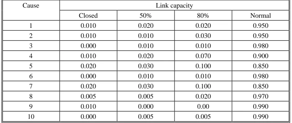
[image:16.595.67.525.523.708.2]50% of normal capacity, (iii) 80% of normal capacity, and (iv) completely closed. For simplicity, the probability of each link to take one of the four modes are the same for all links under the same cause. Table 2 shows the probabilities for each link mode under different causes. As mentioned earlier, the actual number of possible link capacities can be higher than these four pre-defined values, as a result of applying the product operator.
Cause Link capacity
Closed 50% 80% Normal
1 0.010 0.020 0.020 0.950
2 0.010 0.010 0.030 0.950
3 0.000 0.010 0.010 0.980
4 0.010 0.020 0.070 0.900
5 0.020 0.030 0.100 0.850
6 0.000 0.010 0.010 0.980
7 0.020 0.030 0.100 0.850
8 0.005 0.005 0.020 0.970
9 0.010 0.000 0.00 0.990
[image:17.595.62.534.213.412.2]10 0.000 0.005 0.005 0.990
Table 2: List capacity probability adopted in the numerical tests
4.2 Test results
As shown in Figure 3, the first stage is to apply the ORDER-MII algorithm to enumerate the set of most probable scenarios from the causes presented in Table 1. In this test, ORDER-MII is requested to enumerate the most probable scenarios to cover 99% of the probability. After applying ORDER-MII, 89 scenarios are generated (this covers 99% of the total probability). Figure 5 shows the probability of each scenario and the cumulative probability as the number of included scenarios increases. Note that the actual number of all possible scenarios is 1,024.
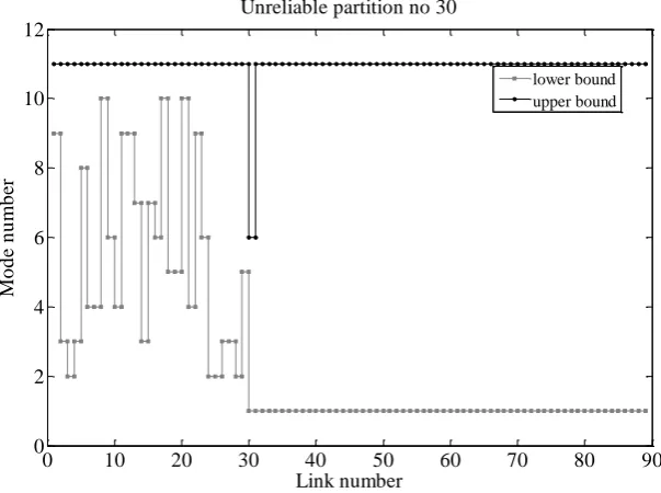
During this process, the set of possible link modes is also obtained. There are in total eleven possible link modes including the normal condition, 80% of capacity, 64% of capacity, 51.2% of capacity, 50% of capacity, 40% of capacity, 32% of capacity, 25% of capacity, 20% of capacity, 12.5% of capacity, and link closed. The next step is then to apply the partition algorithm to generate reliable, unreliable, and undetermined partitions by findingq and s
s j
and (17), can then be defined. Figure 6 shows an example of an unreliable partition defined byq and s
s j
l for link 30. Figure 7 illustrates the progress of the partition algorithm in generating a number of
unreliable partitions and reducing the gap between the upper and lower bounds by accumulating the probability of the unreliable partitions.
10 20 30 40 50 60 70 80
0.00 0.05 0.10 0.15 0.20 0.25 0.30 0.35 0.40 0.45 0.50 0.55 0.60 S c e n a ri o p ro b a b il it y
10 20 30 40 50 60 70 80 0.35
[image:18.595.137.471.198.420.2]0.40 0.45 0.50 0.55 0.60 0.65 0.70 0.75 0.80 0.85 0.90 0.95 1.00 Scenario no. C u m u la ti v e p ro b a b il it y Cumulative probablity Scenario probability
Figure 5: Probability and cumulative probability of scenarios generated by ORDER-MII
0 10 20 30 40 50 60 70 80 90
0 2 4 6 8 10 12
Unreliable partition no 30
Link number Mo d e n u mb er lower bound upper bound
[image:18.595.144.446.481.706.2]0 10 20 30 40 50 60 70 80 90 0 0.002 0.004 0.006 0.008 0.01 0.012 0.014 Partition number P a rt it ion pr oba bi li ty
0 10 20 30 40 50 60 70 80 900 0.05 0.1 0.15 0.2 0.25 0.3 0.35 C um ul a ti ve pr ob of unr e li a bl e pa rt it ions
Cumulative probablity of unreliable partitions
[image:19.595.137.464.86.297.2]Partition probablity
Figure 7: Generated unreliable partitions and their cumulative probability
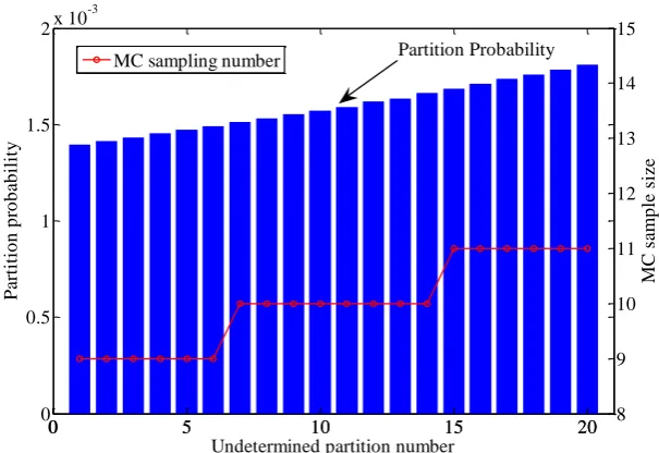
In these tests, 89 undetermined partitions are left after the partition algorithm terminated, which are then passed to the stratified MC algorithm. In the tests, the total number of MC samples is set to be 200. Practically, not all 89 undetermined partitions are sampled, since some of them have negligible probabilities. In the tests, only 20 undetermined partitions are chosen for the stratified MC. Each partition receives the sampling numbers according to its probability. Figure 8 shows the allocation of sample sizes in the MC according to the probability of the partition.
0 5 10 15 20
0 0.5 1 1.5
2x 10
-3 Part it io n p ro b ab il it y
0 5 10 15 20 8
9 10 11 12 13 14 15
Undetermined partition number
MC
samp
le
si
ze
MC sampling number Partition Probability
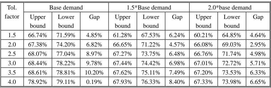
[image:19.595.150.453.496.704.2]Table 3 show the overall test results for three different demand levels and six different tolerance factors.
Tol. factor
Base demand 1.5*Base demand 2.0*base demand Upper
bound
Lower bound
Gap Upper bound
Lower bound
Gap Upper bound
Lower bound
Gap
[image:20.595.65.540.115.269.2]1.5 66.74% 71.59% 4.85% 61.28% 67.53% 6.24% 60.21% 64.85% 4.64% 2.0 67.38% 74.20% 6.82% 66.65% 71.22% 4.57% 66.08% 69.03% 2.95% 2.5 68.07% 77.04% 8.97% 67.27% 73.75% 6.48% 66.76% 71.74% 4.98% 3.0 68.44% 78.22% 9.78% 67.44% 74.42% 6.98% 67.01% 72.72% 5.71% 3.5 68.61% 78.81% 10.20% 67.62% 75.11% 7.49% 67.20% 73.53% 6.33% 4.0 78.92% 79.11% 0.19% 67.93% 76.33% 8.40% 67.33% 73.98% 6.65% Table 3: Upper and lower bounds and gap between the bounds of reliability index (in percentage) with
three demands and six tolerance factors
From the results, with the base demand condition the reliability index of the network is about 66.74% - 71.59%. As the level of the demand increases, it is obvious that the reliability index gradually drops. As expected, the reliability index increases as the tolerance factor increases. However, it is found that the tolerance factor has less effect on the reliability index under the higher demand condition (at least within the given range of the tests).
5. Conclusions
in some theoretical study but should be a sensible assumption in practice. In addition, with the assumption of the partial user equilibrium assignment (PUE) which was also proposed in this paper this condition can be satisfied under some condition. The partition algorithm requires only the small number of network state evaluations to determine a set of reliable and unreliable partitions. The remaining states are grouped into different undetermined partitions. The algorithm will iteratively dissect the undetermined partitions from the previous iteration into a number of reliable and unreliable partitions and update the upper and lower bounds of the reliability function. After reaching the maximum iteration number, the remaining unreliable partitions will be evaluated by the MC with the stratified sampling technique. The algorithm proposed can actually be applied to a wide range of traffic models (e.g. SUE or micro-simulation) and reliability indices provided that the monotone property of the reliability function under different modeling assumptions are justified.
Acknowledgements
This research was funded by the UK Department for Transport under the New Horizons research programme. The authors also wish to thank Dr. Richard Connors for useful discussions and contributions to this study.
References
Asakura, Y. (1999). Evaluation of network reliability using stochastic user equilibrium. Journal Of Advanced Transportation, 33(2), 147-158.
Asakura, Y., Hato, E., and Kashiwadani, M. (2003). Stochastic network design problem: an optimal link investment model for reliable network. "The Network Reliability of Transport: Proceeding of the 1st International Symposium on Transportation Network Reliability", M. G. H. Bell and Y. Iida, eds., Elsevier, Oxford, UK.
Bell, M. G. H., and Iida, Y. (1997). Transportation Network Analysis, John Wiley & Sons, Chichester, UK.
Berdica, K. (2002). An Introduction to Road Vulnerability. Transport Policy, 9, 117-127.
Chen, A., Yang, H., Lo, H. K., and Tang, W. H. (2002). Capacity reliability of a road network: an assessment methodology and numerical results. Transportation Research, 36B(3), 225-252. Clark, S. D., and Watling, D. P. (2005). Modelling network travel time reliability under stochastic
demand. Transportation Research, 39B(2), 119-140.
Doulliez, P., and Jamoulle, J. (1972). Transportation networks with random arc capacities. RAIRO, Recherche Operationnelle Operations Research, 3, 45-60.
Heydecker, B. G., Lam, W. H. K., and Zhang, N. (2007). Use of travel demand satisfaction to assess road network reliability. Transportmetrica, 3(2), 139-171.
Larsson, T., Lundgren, D., Patriksson, M., and Rydergren, C. "An algorithm for finding the most likely equilibrium route flows." The Third Triennial Symposium on Transportation Analysis, San Juan, Puerto Rico.
Lo, H. K., and Tung, Y. K. (2003). Network with degradable links: capacity analysis and design. Transportation Research, 37B(4), 345-363.
Sumalee, A., and Kurauchi, F. (2006). Network Capacity Reliability Analysis Considering Traffic Regulation after a Major Disaster. Networks and Spatial Economics, 6(3-4), 205-219.
Sumalee, A., and Watling, D. P. (2003). Travel Time Reliability in a Network with Dependent Link Modes and Partial Driver Response. Journal of Eastern Asia Society for Transportation Studies, 5, 1687-1701.
Sumalee, A., Watling, D. P., and Nakayama, S. (2007). Reliable Network Design Problem: the case with uncertain demand and total travel time reliability. Transportation Research Record, 1964, 81-90.
Taylor, M. A. P., Sekhar, S. V. C., and D'Este, G. M. (2006). Application of accessibility based methods for vulnerability analysis of strategic road networks. Networks & Spatial Economics, 6(3-4), 267-291.