Physically Versus
Synthetically Replicated Trackers:
Is There A Difference In Terms Of Risk?
Frantz Maurer, Ph.D., Kedge Business School, France
S. Owen Williams, CFA, DBA, Grenoble Ecole de Management, France
ABSTRACT
This article presents the two methods of constructing exchange traded funds and questions whether investors should privilege one structure over the other. To do so, the authors detail the sources of tracking error and risks inherent in each method. As synthetically-created funds include an additional dimension of risk, the authors seek to determine to what measure investors are compensated for this added risk.
Keywords: Exchange-Traded Funds; Physically Versus Synthetically Replicated Trackers; Tracking Error; Risk
1. INTRODUCTION
he first exchange-listed index funds, commonly known as trackers or ETFs (exchange-traded funds), date from the mid-1990s in the United States. The first European tracker was launched in 2000. One of the major innovations within the realm of financial products, these hybrid funds combine the qualities of traditional index funds and ordinary stocks. As with a traditional fund, a tracker offers portfolio diversification in a single transaction with the inherent cost advantages. Like a stock, ETFs are traded real-time throughout the day at a price determined by supply and demand forces (Madhavan, 2012). Passively managed, tracker funds only seek to mirror the exact performance characteristics as the underlying index.
Given the broad range of ETFs today, usually with several sponsors offering a tracker on the same underlying index, an investor today may ask if there is a difference in choosing one index fund over another (Newlands, 2011). An important criterion to consider in answering this question would be the replication method employed by the fund. Our aim in this article is to show that synthetic ETFs contain additional risk relative to physical ETFs. The interest in the paper is two-fold. From an academic perspective, our findings provide additional insight into the efficiency of exchange-listed investment vehicles. From a practitioner’s point of view, an investor should always choose the investment that maximizes expect return per unit of risk. Notably, it would seem incoherent in an efficient market for two funds to coexist that offer the same return objective, yet with one fund carrying more risk. Therefore, given the differing risk structures among trackers, we seek to determine if and how investors in synthetically-created ETFs are compensated for the additional risk inherent in this method of construction.
The article begins by introducing the two forms of fund construction, noting the potential causes of benchmark error and possible sources of additional compensation for synthetic ETF investors. The following section presents the data and methodology for evaluating tracking efficiency of ETFs. Finally we then interpret the results and offer our conclusion.
2. THE TWO ALTERNATIVE APPROACHES TO ETF CONSTRUCTION
In this section, we first remind readers of the two main issues related to the structure of the ETF. Then, we present the characteristics of physically-replicated ETFs, the predominant structure of U.S.-listed trackers, and then the features of European synthetic trackers.
2.1 Legal Structure and Replication Method
In creating a new index tracker fund, the investment management company (sponsor) makes two important decisions regarding the structure of the ETF. On one hand, the fund must be organized as a specific legal structure, typically either a unit investment trust (an open-end mutual funds) or a grantor trust. On the other hand, the sponsor needs to decide on the replication method. While ETFs are generally organized as unit investment trusts in the U.S., tracker funds in Europe tend to be organized as open-end investment companies with UCITS (Undertakings for Collective Investments in Transferable Securities) status. This European directive, aimed at harmonizing the continent’s financial markets, allows funds to be sold more easily across borders without having to list separately in each country. A particularity of UCITS regulations allows for index funds to resort to derivative products to replicate the underlying index. As a result, European ETF sponsors tend to use a swap-based approach to construct their funds. In contrast, the majority U.S.-listed equity funds, subject to the Investment Company Act of 1940, are limited to a physical replication method1. The choices of legal structure and replication method determine how the fund is administered and influence the precision with which the tracker reproduces its benchmark index.
2.2 Physically Replicated Trackers
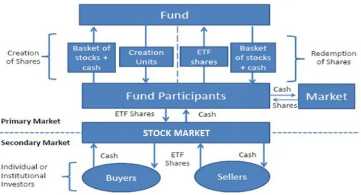
Complete physical replication entails that the investment company purchases all constituent securities of the benchmark index, in the same proportions, for inclusion in the tracker. An ETF on the Dow Jones Eurostoxx 50 index managed physically, for example, would include all fifty securities in order to reproduce all index events. The principal advantage of this technique is the full transparence, as the investor knows with certainty the nature of his/her investment and can see the composition of the fund on a daily basis. The drawback of complete physical replication is the necessity for the fund manager to modify regularly the composition of the tracker following index rebalancings. As full physical replication is relatively expensive in terms of additional commissions, especially for broad indexes composed of hundreds of stocks or for some emerging market indexes containing illiquid components, many sponsors attempt to optimize their cost structure through a variant of full replication. Representative sampling, or optimization, used in cases where full replication is neither cost-effective nor necessary to reproduce the underlying, resorts to investing in only a fraction of the constituent securities. The choice of relevant securities for inclusion in the tracker depends on their market capitalization, as well as fundamental and sector-based criteria, to arrive at an optimal basket. By disregarding relatively illiquid securities with a low index weighting, generally not having a significant impact on fund performance, the fund can effectively reduce costs. The risk in an optimization strategy is omitting a security whose price records an exceptional rise, leading to possibly large tracking errors for the fund. Figure 1 resumes the operational structure for a tracker constructed by physical replication.
1 Sponsors of ETFs not registered under the Investment Company Act of 1940 may resort to the use of derivatives in fund construction. However
Figure 1: Operational Structure Of A Physically Replicated ETF
In contrast to a classic mutual fund, the tracker’s sponsor does not sell shares directly to the public. Instead, large investors, such as investment banks, named authorized participants (AP), play a role as market maker. During share creation, an AP buys the constituent stocks in the tracker directly on the secondary market (whenever ETF shares are significantly overvalued relative to the net asset value), then delivers baskets of these shares, reproducing the exact weightings as the benchmark, along with a cash balance, to the fund. The cash balance represents the amount which equalizes the value of the AP’s creation basket and value of the tracker at the moment of the transaction. In return, the AP receives shares in the ETF, usually in creation units of 50,000 shares. This in-kind transaction, completed on the primary market, physically creates new shares of the tracker. In contrast, synthetic creation, described below, is a cash-only transaction. The shares issued on the primary market are finally brought to the secondary market by the AP for trading. For share redemption, the process is carried out in the other direction. The same APs buy back undervalued tracker shares on the secondary market and deliver these ETF shares to the fund in exchange for shares of the constituent stocks, thereby fulfilling their role as arbitragers.
2.3 Synthetically Replicated Trackers
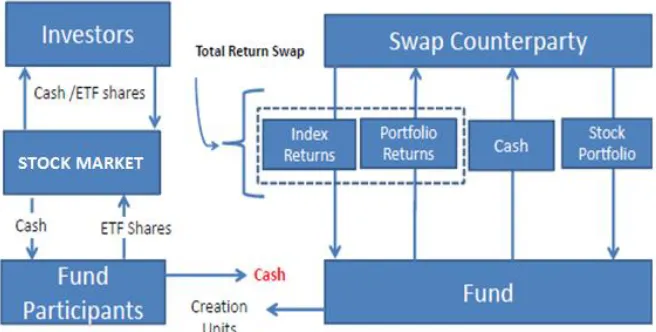
The synthetic method of ETF construction, practiced mainly in Europe, consists of purchasing a collateral basket of stocks, typically a partial replication of the benchmark index, then entering into a swap agreement with a counterparty, such as an investment bank. Through the swap agreement, the fund exchanges the performance of the collateral basket against that of the underlying index, thereby assuring a perfect replication of the benchmark (Dickson et al., 2013; Johnson et al., 2012). The synthetic technique holds several advantages. In principle, this method should offer a tighter fit with respect to the benchmark as the risk of performance deviation is incurred by the counterparty. Moreover, the ETF manager no longer needs to respect the composition of the index since the manager is assured to receive the index performance through the swap agreement. This flexibility creates two sources of added value for the fund – cost reduction and liquidity optimization. These qualities are particularly appreciated in cases where the costs and risks of physical replication are high. A second advantage which stems from the swap-based approach is the ability to reproduce indexes which are too concentrated to respect diversification requirements imposed by regulators. A final reason ETF sponsors employ a synthetic technique in tracker construction is to gain access to certain emerging markets where restrictions are imposed on foreign ownership of local stocks (as in the case for mainland China or India). Figure 2 details the functioning of a synthetically-replicated ETF using an unfunded swap structure2.
2 The corresponding funded swap structure is used less frequently. In this method, the fund sponsor delivers cash to the counterparties who then
Figure 2. Operational Structure Of A Synthetically Replicated ETF
In this method, authorized participants receive creation units in return for cash payments, in lieu of an exchange of securities on the primary market. With the cash, the sponsor acquires the collateral basket of securities from the swap counterparty. The fund then engages in a total return swap with a financial intermediary in order to receive the return on the underlying index (dashed part of figure). Separately, an amount of cash equivalent to the nominal exposure is paid to the counterparty of the swap. In exchange, the swap counterparty transfers a basket of securities to the fund to serve as collateral (right-hand side of figure). A key point is that this collateral basket may be completely different from that of the underlying index. Finally, the total return on collateral basket of securities is then transferred to the swap counterparty.
2.4 Benchmark Risk Factors In Physical And Synthetic Etfs
Whatever method of replication used, the single objective of all ETFs is to reproduce the performance of the underlying index with a minimal tracking error. The sources of this tracking error differ by method of fund construction. Several factors contribute collectively to differentiate the performance of both types of trackers from that of the benchmark. Management fees, cash holdings, and treatment of dividends are three common sources of tracking error. One additional transaction cost, the swap spread, is not reflected in the total expense ratio (TER) of synthetic ETFs and must also be considered. Meanwhile, index revisions, which necessitate fund rebalancing, and optimization issues present unique risks for physical trackers.
Sponsors of synthetic tracks claim that these swap-based funds offer a superior replication of the underlying index. Although the argument is theoretically convincing, several elements may counterbalance the advantage of synthetic ETFs. First, the burden of management fees may vary greatly by fund (Gastineau, 2004), as seen in the TER column in Table 1. Moreover, the additional cost of the swap spread may offset, to some degree, the apparent cost advantage in cases where the synthetic tracker has a lower TER compared to the physical counterpart. A second fund-specific factor to consider is size of the tracker’s cash reserve. A tracker holding more liquidity will tend to underperform a rival fund during up markets and outperform the competitor in down markets. A fund’s dividend policy may also contribute to the cash drag of a tracker3. Yet another equilibrating factor is the
degree to which the fund engages is security lending to generate supplemental revenue for the tracker. With these additional receipts, some trackers offer a nearly perfect replication of the benchmark, despite fees and cash reserves.
Turning to the question of risk, the difference between the two management styles is more distinct. Should the sponsor of a physical ETF default, shareholders simply receive the component stocks in the benchmark. In the other case, as swap-based trackers do not hold the index basket of stocks, the default of a sponsor of a synthetic ETF may result in a significant loss for the ETF shareholders. Moreover, the use of swap agreements with third
3 One example is that of Lyxor ETF, whose managers until 2011 held received dividends in cash before distribution to shareholders of the
parties creates another layer of counterparty risk4. Undeniably, a synthetic ETF presents greater counterparty-risk than physical ETFs. As a result, in efficient markets, an investor should expect to be compensated for holding a synthetic ETF versus a comparable physically-replicated tracker. Compensation for this supplemental risk could come in the form of (i) a lower total expense ratio, thereby offering a greater potential for excess returns, (ii) improved liquidity, or (iii) through a lower relative tracking error.
An inspection of Table 1 reveals that synthetic ETFs are not systematically cheaper in terms of TERs (see the TER column) even before considering the cost of swap spreads. Moreover, using bid-ask spreads as a proxy for liquidity, we observe that it is rather the physically replicated trackers that offer tighter spreads (see the bid/ask column). We must then consider the possibility that the higher risk of synthetic ETFs is compensated for by a superior replication of the benchmark relative to physical ETFs. A test of tracking ability would also seem intuitive as it is reasonable to assume that high fund expenses and poor liquidity would be at least partially reflected in a tracker’s performance relative to its benchmark. The following section presents our dataset and testing methodology to examine the question of tracker efficiency.
3. DATA AND METHODOLOGY
In this section, we deal with the sample selection and explain why we have selected Net Asset Values or NAV data to conduct our empirical analyses. Then, we present the performance tests used to evaluate the efficiency of physical versus synthetic ETFs.
3.1 Sample Selection
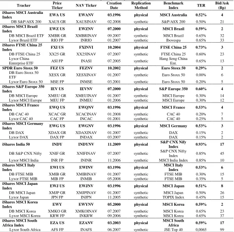
Although ETFs exist for many assets classes, including bonds, commodities, currencies and alternative assets, this paper examines a cross-section of country equity ETFs. To control for management styles, the sample is limited to three fund families: iShares (Blackrock), Lyxor (Société Générale) and db X-trackers (Deutsche Bank). The established physically replicated iShares funds serve as a standard of comparison for the relatively recent synthetic trackers of Lyxor and Deutsche Bank. The forty-nine sample funds, paired by region, are shown in Table 1.
4 Synthetic ETFs attempt to limit risk through the use of multiple counterparties and, in accordance with UCITS regulations, by limiting each
Table 1: Sample Of Physically And Synthetically Replicated ETF
Tracker Price
Ticker NAV Ticker
Creation Date
Replication Method
Benchmark
Index TER
Bid/Ask (Bp) iShares MSCI Australia
Index EWA US EWANV 03.1996 physical MSCI Australia 0.52% 4
DB S&P/ASX 200 XAUS GR XAUSINAV 02.2008 synthetic S&P/ASX 200 0.50% 21 iShares MSCI Brazil
Index EWZ US EWZNV 07.2000 physical MSCI Brazil 0.59% 2
DB MSCI Brazil ETF XMBR GR XMBRINAV 09.2007 synthetic MSCI Brazil 0.65% 32 Lyxor Brazil ETF RIO FP INRIO 01.2007 synthetic Ibovespa 0.65% 33 iShares FTSE China 25
Index FXI US FXINVI 10.2004 physical FTSE China 25 0.73% 3
DB FTSE China 25 XX25 GR XX25INAV 07.2007 synthetic FTSE China 25 0.60% 23 Lyxor China
Enterprise ETF ASI FP INASI 07.2005 synthetic
Hang Seng China
Ent. 0.65% 13
SPDR Euro Stoxx 50 FEZ US FEZNV 10.2002 physical Euro Stoxx 50 0.29% 2
DB Euro Stoxx 50
ETF XESX GR XESXINAV 01.2007 synthetic Euro Stoxx 50 0.00% 6 Lyxor Euro Stoxx 50 MSE FP INMSE 03.2001 synthetic Euro Stoxx 50 0.20% 5 iShares S&P Europe 350
Index IEV US IEVNV 07.2000 physical S&P Europe 350 0.60% 4
DB MSCI Europe XMEU GR XMEUINAV 01.2007 synthetic MSCI Europe 0.30% 14 Lyxor MSCI Europe MEU FP INMEU 01.2006 synthetic MSCI Europe 0.30% 12 iShares MSCI France
Index EWQ US EWQNV 03.1996 physical MSCI France 0.53% 4
DB CAC 40 XCAC GR XCACINAV 01.2008 synthetic CAC 40 0.20% 7 Lyxor CAC 40 CAC FP INCAC 01.2001 synthetic CAC 40 0.25% 5 iShares MSCI Germany
Index EWG US EWGNV 03.1996 physical MSCI Germany 0.53% 3
DB DAX XDAX GR XDAXINAV 01.2007 synthetic DAX 0.15% 2 Lyxor DAX DAX FP INDAX 03.2007 synthetic DAX 0.15% 2
iShares India 50 INDY INDYNV 11.2009 physical S&P CNX Nify
Index 0.93% 17
DB S&P CNX Nifty XNIF GR XNIFINAV 07.2007 synthetic S&P CNX Nifty
Index 0.85% 45 Lyxor MSCI India INR FP ININR 11.2006 synthetic MSCI India Index 0.85% 10 iShares MSCI Italy
Index EWI US EWINV 03.1996 physical
MSCI Italy
Index 0.53% 6
DB FTSE MIB XMIB GR XMIBINAV 01.2007 synthetic FTSE MIB 0.30% 15 Lyxor FTSE MIB MIB FP INMIB 05.2008 synthetic FTSE MIB 0.35% 5 iShares MSCI Japan
Index EWJ US EWJNV 03.1996 physical MSCI Japan 0.51% 8
DB MSCI Japan XMJP GR XMJPINAV 01.2007 synthetic MSCI Japan 0.50% 26 Lyxor Japan JPN FP INJPN 11.2005 synthetic TOPIX Index 0.45% 15 iShares MSCI Korea
Index EWY EWYNV 05.2000 physical MSCI Korea 0.59% 2
DB MSCI Korea XMKO GR XMKOINAV 07.2007 synthetic MSCI Korea 0.65% 23 Lyxor MSCI Korea KRW FP INKRW 09.2006 synthetic MSCI Korea 0.65% 37 iShares MSCI South
Africa Index EZA US EZANV 03.2003 physical
MSCI South
Africa 0.59% 17
(Table 1 continued)
Tracker Price
ticker NAV ticker
Creation date
Replication method
Benchmark
Index TER
Bid/ask (bp) iShares MSCI Spain
Index Fund EWP US EWPNV 03.1996 physical MSCI Spain 0.53% 8
Lyxor IBEX 35 ETF LYXIB SM INLYXIB 10.2006 synthetic IBEX 0.30% 16 iShares MSCI
Switzerland Index Fund EWL US EWLNV 03.1996 physical
MSCI
Switzerland 0.53% 3
DB SMI ETF XSMI GR XSMIINAV 01.2007 synthetic Swiss Market
Index 0.30% 12 iShares MSCI Taiwan
Index Fund EWT US EWTNV 06.2000 physical MSCI Taiwan 0.59% 7
DB MSCI Taiwan
ETF XMTW GR XMTWINAV 07.2007 synthetic MSCI Taiwan 0.65% 41 Lyxor Taiwan ETF TWN FP INTWN 03.2008 synthetic MSCI Taiwan 0.65% 45 iShares MSCI Turkey
Index Fund TUR US INAVTUKP 03.2008 physical MSCI Turkey 0.59% 2
Lyxor Turkey ETF TUR FP INTUR 08.2006 synthetic DJ Turkey
Titans 20 0.65% 41 iShares MSCI United
Kingdom Fund EWU US EWUNV 03.1996 physical
MSCI United
Kingdom 0.53% 5
DB FTSE 100 ETF XUKX GR XUKXINAV 06.2007 synthetic FTSE 100 0.30% 18 Lyxor FTSE 100 ETF L100 FP IN100 05.2008 synthetic FTSE 100 0.15% 8 iShares S&P 500 Fund IVV US IVVNV 05.2000 physical S&P 500 0.07% 1 DB MSCI USA ETF XMUS GR XMUSINAV 01.2007 synthetic MSCI USA 0.30% 21 Lyxor MSCI USA USA FP INUSA 03.2006 synthetic MSCI USA 0.30% 14 Note. The established physically replicated iShares funds are displayed in bold. TER denotes the Total Expense Ratio. Bid/ask denotes the bid-ask spreads (expressed in basis point) and is used as a proxy for liquidity.
3.2 Net Asset Value (NAV) Data
The analysis is carried out on fund NAVs and each series is truncated from the end of Q1 2008 to December 31, 20135. Net asset values are used to eliminate price variations due to market noise and other non-fundamental factors, including time zone effects. The net asset value (NAV) for the fund using the market value of component stocks is published each day at the close of trading and defined as follows:
Analysis of NAVs remains pertinent for the investor, as Gastineau (2001) demonstrates that any divergence between price and NAV is eliminated over the long-term by the creation/redemption process. We use net asset values in this paper as we believe this measure gives the best indication of the performance of a tracker relative to its benchmark index, without compromising the relevance of this study for investors. Representing the fair value of assets in the fund, the NAV does not fluctuate based on investor emotion. Meanwhile, a tracker’s price is very sensitive to domestic market risk factors (especially in the case of a country ETF) and to supply/demand disequilibrium (Zhong and Yang, 2005). While the previous research on ETFs consider price data, our study is among to first to analyze the NAV prices of country trackers.
Next, dividends are added back to the fund values on the ex-dates in order to compare trackers to the total return benchmark indexes. Finally, to control for the exchange rate effect, the common currency indexes are used. We collected all raw tracker price data directly from the fund providers while raw benchmark index data came from the Bloomberg database. Each data series is finally transformed into daily returns by taking the first difference of log prices assuming continuous compounding.
3.2 Performance Tests
The study employs several methods to evaluate the relative efficiency of physical and synthetic ETFs. We first quantify ETF deviations from the benchmark by measuring the tracking errors of returns. Following the approach of Milonas and Rompotis (2010) and Shin and Soydemir (2010), we apply three different calculations then take the mean of these tracking errors. The first tracking error (TE) is the mean of absolute differences between ETF and benchmark returns:
(2)
where:
is the tracker’s daily NAV return,
is the benchmark index return.
The second estimation uses the error term of a least squares regression of tracker returns on the index returns:
Here, the alpha coefficient ( i), which indicates the excess return of the ETF, and the beta coefficient ( i), which represents the systematic risk, should approach zero and unity, respectively, for a well-constructed tracker. Therefore, the regression residual ( i,t) will give us an estimation of the fund’s tracking error. If the index replication is perfect, the standard deviation of residuals should equal zero.
The last measure of tracking error is given by the standard deviation of return differences between the ETF and its underlying benchmark:
Here, ei,t is the difference in returns between the tracker NAV and the index on day t. If the ETF correctly reproduces the index returns, the mean of these three measures should approach zero.
Since tracking error does not fully capture the volatility of returns (Johnson, 2009; Chen et al., 2006), we extend the study by analyzing the Sortino, Omega, and modified Sharpe ratios. Unlike the traditional Sharpe ratio, the Sortino and Omega ratios uses downside deviation instead of standard error (Sortino and Price, 1994; Keating and Shadwick, 2002). Both these risk-adjusted performance measures, which take into account asymmetry and extreme risks, are based on the use of lower partial moments. Used frequently in the hedge fund industry due to the non-normal character of strategy returns, the Sortino and Omega calculations should approximate the Sharpe ratio (Eling and Schuhmacher, 2007). In order to adapt the Sortino to the current analysis, the benchmark returns are substituted in place of the required return:
Where:
The calculation therefore offers a risk-adjusted performance measure which does not penalize the tracker for upside price variations (positive tracking error). The Omega ratio gives an alternative look at the volatility of a tracker relative to its index. Unlike other risk measures, the Omega ratio considers all moments of the distribution:
where:
(a, b) is the interval of returns, r is the loss threshold,
and F is the cumulative distribution of returns.
As for the Sortino, the benchmark serves as the reference point, taking the value of in the Omega estimation. This ratio will be equal to unity when the loss threshold nears the mean return on the asset, indicating a similar risk profile between the tracker and the benchmark index.
Lastly, we use a modified Sharpe ratio, where volatility is replaced by a value-at-risk (VaR) estimate, to allow comparisons across funds under a scenario of negative excess returns. The modified Sharpe gives the ratio of excess tracker returns over the benchmark divided by the modified VaR:
The modified value-at-risk (MVaRp), based on a Cornish-Fisher expansion where risk is measured by standard
deviation, skewness, and kurtosis at a given confidence level (p), is similar to the classical VaR but will be worse in cases where the tracker posts extreme negative returns relative to the benchmark (Favre and Galeano, 2002). The confidence level is set to 95% for our calculations.
4. EMPIRICAL RESULTS AND DISCUSSION
In this section, we discuss the main results provided by the analysis of tracking error. Supported by our main empirical findings, we then suggest a risk-based international ETF investment strategy.
4.1 Analysis of Tracking Error
Table 2: iShares Funds, Performance Measures (31 March, 2008 – 31 December, 2013) Country
Index Fund
Mean Return
Tracking Error 1
Tracking Error 2
Tracking Error 3
Mean
Error Sortino Omega
Modified Sharpe N iShares MSCI
Australia Fund 0.0180 0.4907 0.0063 0.7961 0.4310 0.0009 1.0029 0.0007 1421 iShares MSCI Brazil
Fund -0.0035 0.3550 0.0089 0.5551 0.3063 0.0054 1.0166 0.0040 1390 iShares FTSE China
25 Fund -0.0033 0.0493 0.0007 0.5205 0.1902 0.0067 1.1655 -0.0422 1384 SPDR Euro Stoxx
50 Fund 0.0049 0.3375 0.0029 0.4814 0.2739 -0.0033 0.9908 -0.0019 1442 iShares S&P Europe
350 Fund 0.0154 0.3285 0.0062 0.4720 0.2689 0.0032 1.0092 0.0019 1442 iShares MSCI
France Fund 0.0094 0.3425 0.0053 0.4873 0.2784 0.0003 1.0008 0.0002 1438 iShares MSCI
Germany Fund 0.0206 0.3397 0.0110 0.4829 0.2778 0.0007 1.0020 0.0004 1429 iShares MSCI India
Fund 0.0248 0.3695 0.0198 0.5213 0.3035 0.0049 1.0130 0.0032 991 iShares MSCI Italy
Fund -0.0214 0.3523 0.0120 0.4917 0.2853 -0.0015 0.9959 -0.0009 1425 iShares MSCI Japan
Fund 0.0092 0.3167 0.0065 0.4899 0.2710 0.0048 1.0153 0.0030 1365 iShares MSCI Korea
Fund 0.0183 0.4438 0.0025 0.7453 0.3972 0.0023 1.0076 0.0019 1192 iShares MSCI South
Africa Fund 0.0427 0.5913 0.0122 0.9512 0.5182 0.0035 1.0106 -0.0015 1402 iShares MSCI Spain
Fund 0.0011 0.3574 0.0131 0.5024 0.2910 -0.0076 0.9790 -0.0046 1433 iShares MSCI
Switzerland Fund 0.0177 0.3626 0.0154 0.5170 0.2983 -0.0014 0.9960 -0.0009 1413 iShares MSCI
Taiwan Fund 0.0047 0.1422 0.0033 0.2836 0.1430 0.0068 1.0280 -0.0014 1381 iShares MSCI
Turkey Fund 0.0445 0.2719 0.0084 0.4455 0.2419 0.0051 1.0160 0.0041 1398 iShares MSCI United
Kingdom Fund 0.0244 0.3032 0.0104 0.4333 0.2490 0.0056 1.0159 0.0035 1422 iShares S&P 500
Fund 0.0317 0.0029 0.0001 0.0087 0.0039 0.0169 1.1146 -0.0005 1450
Global Descriptive Statistics
Mean 0.0144 0.3198 0.0081 0.5103 0.2794 0.0030 1.0211 -0.0017 1379
Median 0.0166 0.3411 0.0075 0.4908 0.2781 0.0034 1.0099 0.0003 1417
Minimum -0.0214 0.0029 0.0001 0.0087 0.0039 -0.0076 0.9790 -0.0422 991
Maximum 0.0445 0.5913 0.0198 0.9512 0.5182 0.0169 1.1655 0.0041 1450
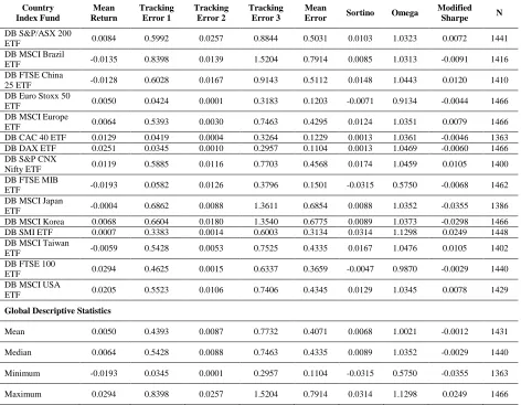
Table 3: Deutsche Bank Funds, Performance Measures (31 March, 2008 – 31 December, 2013)
Country Index Fund
Mean Return
Tracking Error 1
Tracking Error 2
Tracking Error 3
Mean
Error Sortino Omega
Modified
Sharpe N
DB S&P/ASX 200
ETF 0.0084 0.5992 0.0257 0.8844 0.5031 0.0103 1.0323 0.0072 1441 DB MSCI Brazil
ETF -0.0135 0.8398 0.0139 1.5204 0.7914 0.0085 1.0313 -0.0091 1416 DB FTSE China
25 ETF -0.0128 0.6028 0.0167 0.9143 0.5112 0.0148 1.0443 0.0120 1410 DB Euro Stoxx 50
ETF 0.0050 0.0424 0.0001 0.3183 0.1203 -0.0071 0.9134 -0.0044 1466 DB MSCI Europe
ETF 0.0064 0.5393 0.0030 0.7463 0.4295 0.0124 1.0351 0.0079 1466 DB CAC 40 ETF 0.0129 0.0419 0.0004 0.3264 0.1229 0.0013 1.0361 -0.0046 1363 DB DAX ETF 0.0251 0.0345 0.0010 0.2957 0.1104 0.0013 1.0469 -0.0060 1466 DB S&P CNX
Nifty ETF 0.0119 0.5885 0.0116 0.7703 0.4568 0.0174 1.0459 0.0105 1400 DB FTSE MIB
ETF -0.0193 0.0582 0.0126 0.3796 0.1501 -0.0315 0.5750 -0.0068 1462 DB MSCI Japan
ETF -0.0004 0.6862 0.0088 1.3611 0.6854 0.0088 1.0352 -0.0355 1386 DB MSCI Korea 0.0068 0.6604 0.0180 1.3540 0.6775 0.0089 1.0373 -0.0298 1466 DB SMI ETF 0.0007 0.3383 0.0014 0.6003 0.3134 0.0314 1.1298 0.0249 1448 DB MSCI Taiwan
ETF -0.0059 0.5428 0.0053 0.7525 0.4335 0.0167 1.0476 0.0105 1402 DB FTSE 100
ETF 0.0294 0.4625 0.0015 0.6337 0.3659 -0.0047 0.9870 -0.0029 1440 DB MSCI USA
ETF 0.0205 0.5523 0.0106 0.7406 0.4345 0.0129 1.0345 0.0078 1429
Global Descriptive Statistics
Mean 0.0050 0.4393 0.0087 0.7732 0.4071 0.0068 1.0021 -0.0012 1431
Median 0.0064 0.5428 0.0088 0.7463 0.4335 0.0089 1.0352 -0.0029 1440
Minimum -0.0193 0.0345 0.0001 0.2957 0.1104 -0.0315 0.5750 -0.0355 1363
Maximum 0.0294 0.8398 0.0257 1.5204 0.7914 0.0314 1.1298 0.0249 1466
Table 4: Lyxor Funds, Performance Measures (31 March, 2008 – 31 December, 2013) Country
Index Fund
Mean Return
Tracking Error 1
Tracking Error 2
Tracking Error 3
Mean
Error Sortino Omega
Modified
Sharpe N
Lyxor Brazil ETF -0.0166 0.6002 0.0118 0.9641 0.5254 0.0050 1.0157 0.0039 1415
Lyxor China
Enterprise ETF -0.0007 0.3439 0.0118 0.5004 0.2853 0.0104 1.0306 0.0073 1411 Lyxor Euro Stoxx
50 0.0054 0.0173 0.0012 0.0454 0.0213 -0.0433 0.7653 -0.0005 1467 Lyxor MSCI
Europe ETF 0.0153 0.0113 0.0000 0.0431 0.0181 0.0063 1.0578 -0.0014 1468 Lyxor CAC 40
ETF 0.0090 0.0129 0.0001 0.0316 0.0149 0.0306 1.2171 0.1476 1476
Lyxor DAX ETF 0.0244 0.0118 0.0004 0.0953 0.0359 0.0129 1.2957 -0.0058 1466
Lyxor MSCI India
ETF 0.0189 0.4238 0.0067 0.5812 0.3372 0.0081 1.0225 0.0053 1399 Lyxor FTSE MIB
ETF 0.0292 0.0906 0.0033 0.6544 0.2495 -0.0005 0.9921 -0.0172 1217
Lyxor Japan ETF 0.0101 0.4158 0.0052 0.6637 0.3616 0.0047 1.0158 0.0032 1389
Lyxor MSCI Korea 0.0174 0.3963 0.0102 0.6949 0.3671 0.0033 1.0121 0.0032 1403
Lyxor South Africa
ETF 0.0363 0.4623 0.0211 0.7682 0.4172 0.0063 1.0193 -0.0076 1388
Lyxor IBEX 35 -0.0018 0.0085 0.0001 0.0304 0.0130 0.0202 1.1853 -0.0015 1470
Lyxor Taiwan ETF 0.0034 0.3561 0.0125 0.4985 0.2890 0.0072 1.0209 0.0047 1344
Lyxor Turkey ETF 0.0469 0.3235 0.0165 0.4958 0.2786 0.0073 1.0220 0.0051 1417
Lyxor FTSE 100 0.0218 0.7728 0.0404 1.5563 0.7898 0.0029 1.0117 0.0027 1452
Lyxor MSCI USA 0.0300 0.3492 0.0075 0.5300 0.2956 -0.0001 0.9998 -0.0001 1438
Global Descriptive Statistics
Mean 0.0156 0.2873 0.0093 0.5096 0.2687 0.0051 1.0427 0.0093 1414
Median 0.0164 0.3466 0.0071 0.5152 0.2872 0.0063 1.0201 0.0030 1416
Minimum -0.0166 0.0085 0.0000 0.0304 0.0130 -0.0433 0.7653 -0.0172 1217
Maximum 0.0469 0.7728 0.0404 1.5563 0.7898 0.0306 1.2957 0.1476 1476
Note. The table presents summary statistics for the Lyxor funds. The first column gives the mean daily return over the period. Tracking error 1 is the mean of absolute differences (equation 2), tracking error 2 gives the regression error term (equation 3) while tracking error 3 corresponds to the standard deviation of return differences (equation 4). The fifth column takes the mean of the three tracking errors. Colu mns six, seven and eight present the results of the tests using the Sortino ratio (equation 5), the Omega ratio (equation 6), and the modified Sharpe measure (Equation 7). The number of daily observations per sample fund is shown in the last column.
At the country level, we find a currency zone effect impacting fund performance. Country funds domiciled in Europe (Lyxor and Deutsche Bank funds) which track a euro zone benchmark index generally offer a significantly smaller mean tracking error in comparison to the U.S.-domiciled iShare funds on the European indexes. Similarly, the iShares S&P 500 fund on New York shows a significantly smaller mean error (0.0039) compared with the Deutsche Bank (0.4345) and Lyxor (0.2956) funds which attempt to track U.S. dollar-listed stocks. This currency zone effect is also apparent with the trackers on the China and Taiwan indexes, with the dollar-listed iShares FTSE China fund and iShares MSCI Taiwan producing a relatively lower tracking error. Again, an authorized participant would incur less risk arbitraging underlying securities in Hong Kong or Taiwanese dollars for subsequent delivery to a fund in U.S. dollars rather than delivery in euros6.
6 The Hong Kong Monetary Authority maintains a currency board against the U.S. dollar while the Taiwan dollar is unofficially pegged to the
Table 5: Wilcoxon Tests Of Statistical Differences
Tracking Error Sortino Ratio Omega Ratio Modified Sharpe
Region iShare vs.
DB iShares vs. Lyxor iShare vs. DB iShares vs. Lyxor iShare vs. DB iShare vs. Lyxor iShare vs. DB iShares vs. Lyxor
Australia 0.312 - 0.042* - 0.048* - 0.112 -
Brazil 0.013* 0.033* 0.085 0.115 0.071 0.365 0.099 0.401
China 0.041* 0.154 0.038* 0.076 0.026* 0.002** 0.008** 0.002** Eurostoxx 50 0.048* 0.035* 0.231 0.001** 0.037* 0.026* 0.325 0.197
Europe 0.087 0.023* 0.048* 0.068 0.182 0.031* 0.238 0.056 France 0.035* 0.029* 0.199 0.015* 0.221 0.008** 0.332 0.008**
Germany 0.038* 0.011* 0.215 0.019* 0.142 0.006** 0.198 0.010*
India 0.109 0.421 0.033* 0.078 0.201 0.132 0.298 0.066
Italy 0.042* 0.268 0.001** 0.183 0.000** 0.286 0.274 0.018*
Japan 0.008** 0.168 0.162 0.568 0.120 0.341 0.026* 0.255
Korea 0.031* 0.398 0.071 0.412 0.098 0.156 0.035* 0.287
South Africa - 0.114 - 0.050 - 0.064 - 0.048*
Spain - 0.019* - 0.007** - 0.000** - 0.057
Switzerland 0.596 - 0.001** - 0.009** - 0.045* -
Taiwan 0.021* 0.061 0.031* 0.235 0.135 0.100 0.165 0.044*
Turkey - 0.333 - 0.079 - 0.221 - 0.222
United Kingdom 0.156 0.003** 0.026* 0.086 0.184 0.218 0.129 0.310
United States 0.009** 0.005** 0.263 0.012* 0.051 0.008** 0.087 0.467
Global Descriptive Statistics
Mean 0.069 0.291 0.041* 0.049* 0.071 0.088 0.218 0.039*
Median 0.075 0.302 0.037* 0.047* 0.042* 0.074 0.235 0.041* Note. The table presents the p-values from the Wilcoxon tests of statistical differences between iShares funds and Deutsche Bank funds and between iShares funds and Lyxor funds. The tracking error column considers the mean tracking error score for each sample fund. The null hypothesis of the test, H0, is for no difference between the two funds calculated statistic. *signals rejection at the 5% level and **signals rejection
at the 1% level.
On the risk side of the equation, the physically-replicated iShares funds tend to show the least volatility with respect to the benchmark index. The overall mean and median differences between the Sortino risk measures on the iShares and Deutsche Bank funds as well as between the iShares and Lyxor funds are significant at the 5% level (Table 5). The tests using the Omega ratio on the means and medians are significant at the 10% level while the differences using the modified Sharpe measure are only significant against the means and medians for the Lyxor funds. Much of the excess variation within the Lyxor funds is due to the non-reinvestment of dividends prior to 2011. A subsample of data from 2011 to 2013 confirms that return volatility fell after the change in dividend treatment7.Interestingly, among emerging market funds where replication is more difficult due to poorer liquidity in the underlying shares, the physically-constructed iShares tend to display less benchmark risk. Considering the three risk measures in aggregate, the iShares China, India, South Africa, Korea and Taiwan funds all tend to outperform their synthetically-constructed counterparts (Table 5).
4.2 A Risk-Based International ETF Investment Strategy
In selecting a country tracker fund, an investor should consider the tracking error, the benchmark risk (or excess volatility) and the overall fund risk. Our analysis of tracking error suggests that both physical and synthetic ETFs offer, on aggregate, a similar return performance relative to the benchmark. However, difficulties in carrying out arbitrage on underlying shares in currencies different from the fund currency argue in favor of using domestic funds when possible. As such, the iShares S&P 500 is more efficient in tracking U.S. stocks while the Deutsche Bank and Lyxor funds provide a tighter relationship with the indexes in the euro zone. Concerning developing market funds, synthetic fund sponsors argue that swap-based ETFs are better suited to reproduce these emerging market indexes8. Again, our results refute this assertion. Of the seven emerging countries studied, the physical trackers offer a superior risk-adjusted tracker error for four countries (Brazil, China, Korea, and Taiwan) while the error differences are not statistically significant at the 5% level in the remaining cases (Table 5). The results of our
7 To save space, these results are not reproduced here but are available upon request from the authors.
8 Synthetically created funds may have a comparative advantage in tracking certain hard to access markets, such as the China A-shares, where
tracking error analysis, coupled with our previous finding that none of the fund families distinguish themselves in terms of lower expenses or greater liquidity, argue that ETF selection should be made on an ad hoc, fund-by-fund basis.
The risk criteria, meanwhile, tend to favor the physically-constructed iShares funds. In regards to excess volatility relative to the benchmark index, a slight majority of iShares funds show lower risk in comparison to their Deutsche Bank and Lyxor counterparts. Nonetheless, in many cases the Sortino, Omega and modified Sharpe measures are mixed or the differences are not statistically significant. As an investment decision cannot be made based solely on these benchmark risk measures, an investor must also consider overall fund risk. Overall fund risk includes notably the fund’s method of construction. On this metric, synthetically-constructed funds clearly present greater risk, as demonstrated above. The use of physical ETFs, therefore would allow an investor to improve his risk-adjusted ETF returns, where risk considers both explicit risks (excess volatility to benchmark) and implicit risks (default of a swap counterparty).
5. CONCLUSION
This paper attempts to differentiate between the risk/return characteristics of competing physically and synthetically-constructed country ETFs on similar indexes. Our analysis shows that physical ETFs replicate the performance of the underlying benchmarks with, in aggregate, a similar efficiency as synthetic trackers. In addition, using the total expense ratio and average bid-ask spreads as proxies for cost structure and market liquidity, respectively, we do not find a significant advantage in favor of either fund style. Therefore, our study is not able to demonstrate conclusively that investors are compensated for any additional risk inherent in synthetic funds. Although limitations of the size of swap contracts and the use of multiple counterparties reduce the risk inherent in synthetic trackers, the market does not appear to price in any residual risk. We conclude that benchmark-oriented managers and investors investing over longer horizons are generally better advised to use physical ETFs.
AUTHORS’ INFORMATION
Frantz Maurer (corresponding author) is Professor of finance at KEDGE Business School. He holds a Ph.D in Management Science and a post-doctoral degree from the University of Bordeaux. Frantz is the author of several publications directed to academics and practitioners. His current research interests focus primarily on financial risk management in the banking industry. Contact Information: KEDGE Business School, 680 cours de la Libération, 33405 Talence cedex (France). Telephone: +33 (0) 556 845 573.
Email: [email protected].
Owen Williams is a doctoral fellow and visiting professor at Grenoble Ecole de Management. He holds a DBA in finance from Grenoble and is a CFA charterholder. His current research interests include international finance, currency markets, portfolio management, and asset pricing. Contact Information: Grenoble Ecole de Management, 12 rue Pierre Sémard, 38000 Grenoble (France). Telephone: +33 (0) 450251273. Email:
REFERENCES
1. Chen, H., Noronha, G., & Singal, V. (2006). Index Changes and Losses to Index Fund Investors. Financial Analysts Journal, 62(4), 31-47.
2. Dickson, J., Mance, L., & Rowley, J. (2013). Understanding Synthetic ETFs. Vanguard, 15p. Retrieved from https://pressroom.vanguard.com/content/nonindexed/6.14.2013
3. Eling, M., & Schuhmacher, F. (2007). Does the Choice of Performance Measure Influence the Evaluation of Hedge Funds. Journal of Banking and Finance, 31(9), 2632-2647.
4. Favre, L. & Galeano, J.-A. (2002). Mean-Modified Value-at-Risk Optimization with Hedge Funds. Journal of Alternative Investments, 5(2), 21-26.
6. Gastineau, G. (2004). Protecting Fund Shareholders from Costly Trading. Financial Analysts Journal, 60(3), 22-32.
7. Johnson, B, Bioy, H., Choy, J., & Gabriel, J. (2012). Synthetic ETFs Under the Microscope: A Global Study. Morningstar, 63p. Retrieved from Media.morningstar.com/eu/ETF/assets
8. Johnson, W. (2009). Tracking Errors of Exchange Traded Funds. Journal of Asset Management, 10(4), 253–262.
9. Keating, C., & Shadwick, W. (2002). A Universal Performance Measure. Journal of Performance Measurement 6(3), 59-84.
10. Madhavan, A. (2012). Exchange-Traded Funds, Market Structure, and the Flash Crash. Financial Analysts Journal, 68(4), 20-35.
11. Milonas, N., & Rompotis, G. (2010). Dual Offerings of ETFs on the Same Stock Index: US vs. Swiss ETFs. The Journal of Alternative Investments, 12(4), 97–113.
12. Newlands, C. (2011). Physical vs Synthetic Debate is Hotting Up. Financial Times, 6 February, p8. 13. Shin, S., & Soydemir, G. (2010). Exchange-Traded Funds, Persistence in Tracking Errors and Information
Dissemination. Journal of Multinational Financial Management, 20(4-5), 214–234.
14. Sortino, F., & Price, L. (1994). Performance Measurement in a Downside Risk Framework. Journal of Investing, 3(3), 59-64.