Efficient Image-Based Localization Using Context

(1)

Efficient Image-Based Localization Using

Context

by

Charbel Azzi

A thesis

presented to the University of Waterloo in fulfillment of the

thesis requirement for the degree of Master of Applied Science

in

Systems Design Engineering

Waterloo, Ontario, Canada, 2015

(2)

Author’s Declaration

This thesis consists of material all of which I authored or co-authored: see Statement of Contributions included in the thesis. This is a true copy of the thesis, including any required final revisions, as accepted by my examiners.

(3)

Statement of Contributions

This thesis consists of material all of which I co-authored: The work documented in Chap-ter 5 has been submitted to the CompuChap-ter Vision and PatChap-tern Recognition (CVPR), 2016 IEEE Conference. Co-authors include: Charbel Azzi, John Zelek, Daniel Asmar and Adel Fakih. I hereby verify that I am the principal author. Also, the work documented in Chapters 2 and 4 will be submitted to Robotics and Automation Magazine, 2016 IEEE. Co-authors include: Charbel Azzi, John Zelek, Daniel Asmar and Adel Fakih. I hereby verify that I will be the principal author.

(4)

Abstract

Image-Based Localization (IBL) is the problem of computing the position and orientation of a camera with respect to a geometric representation of the scene. A fundamental building block of IBL is searching the space of a saved 3D representation of the scene for correspondences to a query image. The robustness and accuracy of the IBL approaches in the literature are not objective and quantifiable.

First, this thesis presents a detailed description and study of three different 3D modeling packages based on SFM to reconstruct a 3D map of an environment. The packages tested are VSFM, Bundler and PTAM. The objective is to assess the mapping ability of each of the tech-niques and choose the best one to use for reconstructing the IBL 3D map. The study results show that image matching which is the bottleneck of SFM, SLAM and IBL plays the major role in favour of VSFM. This will result in using wrong matches in building the 3D map. It is crucial for IBL to choose the software that provides the best quality of points,i.e.the largest number of correct 3D points. For this reason, VSFM will be chosen to reconstruct the 3D maps for IBL.

Second, this work presents a comparative study of the main approaches, namely Brute Force Matching, Tree-Based Approach, Embedded Ferns Classification, ACG Localizer, Keyframe Approach, Decision Forest, Worldwide Pose Estimation and MPEG Search Space Reduction. The objective of the comparative analysis was to first uncover the specifics of each of these techniques and thereby understand the advantages and disadvantages of each of them. The testing was performed on Dubrovnik Dataset where the localization is determined with respect to a 3D cloud map which was computed using a Structure-from-Motion approach. The study results show that the current state of the art IBL solutions still face challenges in search space reduction, feature matching, clustering, and the quality of the solution is not consistent across all query images.

Third, this work addresses the search space problem in order to solve the IBL problem. The Gist-based Search Space Reduction (GSSR), an efficient alternative to the available search space solutions, is proposed. It relies on GIST descriptors to considerably reduce search space and computational time, while at the same exceeding the state of the art in localization accuracy. Experiments on the 7 scenes datasets of Microsoft Research reveal considerable speedups for GSSR versus tree-based approaches, reaching a 4 times faster speed for the Heads dataset, and reducing the search space by an average of 92% while maintaining a better accuracy.

(5)

Acknowledgements

I would like to thank my supervisor Dr John Zelek. His insight and guidance have made my study exciting, and led this thesis to intriguing places.

I would also like to thank Dr Daniel Asmar. His continuous advice guidance and feedback lead to me to accomplish this work.

I extend many thanks to my reader Dr Steve Waslander for his valued feedback.

Special thanks to Dr Adel Fakih for his advice, support and hands-on help that he provided throughout this thesis.

To Bank Audi who funded my expenses throughout this degree I would like to thank you a lot for believing in me. I would not have accomplished this work without your full support. I will always owe you for the opportunities you have given me.

I would like to thank Ontario Centres of Excellence(OCE) and Natural Sciences and Engi-neering Research Council(NSERC) for funding this project and making it possible.

Finally my ultimate thanks goes to my family for the spiritual support they gave me by always motivating me to overcome the hardships I faced. Without them I would have never achieved this work.

(6)

(7)

List of Tables

3.1 Main algorithmic differences for each package. . . 40

4.1 Area of contributions for the main approaches in IBL . . . 42

4.2 The major datasets used in IBL . . . 49

4.3 Results on Dubrovnik dataset for the provided main approaches . . . 52

4.4 Results taken from the corresponding papers of the non-available approaches . . 52

5.1 The 7 scenes dataset by Microsoft research . . . 65

5.2 GSSR performance benchmarked against the tree-based approach . . . 70

5.3 GSSR performance versus tree-based, Decision Forest, and Keyframe approaches 70 5.4 Search space reduction efficiency of GSSR . . . 72

(11)

List of Figures

2.1 Image-Based Localization Main Components . . . 11

3.1 Reconstructed 3D sparse maps for Jbeil Roman Theatre . . . 31

3.2 Reprojection error Vs feature ID associated for Jbeil Roman Theatre . . . 32

3.3 Reconstructed 3D sparse maps for UW Robotics Lab . . . 33

3.4 Reprojection error Vs feature ID associated for UW Robotics Lab . . . 34

3.5 Reconstructed 3D sparse maps for UW Engineering 5 (E5) Building . . . 36

3.6 Reprojection error Vs feature ID associated for UW E5 building . . . 37

4.1 Decision Forest Pose IBL System. (Shotton et al., 2013) . . . 47

4.2 Vocabulary-based Prioritized Search(VPS). (Sattler et al., 2011) . . . 48

4.3 Active Search System. (Sattler et al., 2012) . . . 48

5.1 GSSR System . . . 56

5.2 GIST descriptor computation.(Torralba et al.,2006) . . . 58

5.3 Inputs into the GSSR system . . . 61

5.4 3D point cloud map for each scene reconstructed from VSFM [65] . . . 64

5.5 GIST credibility for each scene . . . 68

5.6 Charts showing the average inliers number and the search space reduction . . . . 72 5.7 Tracking of the camera motion for GSSR and tree-based against the ground truth 73

(12)

Nomenclature

Symbol Description

IBL Image-Based Localization

GSSR GIST-based Search Space Reduction

2D-2D Two dimensional Space to two dimensional space matching 2D-3D Two dimensional Space to three dimensional space matching

(13)

Acronyms

SLAM Simultaneous Localization And Mapping

KF Keyframe

BA Bundle Adjustment

RT Re-Triangulation

AR Augmented Reality

FLANN Fast Library of Approximate Nearest Neighbor

ANN Approximate Nearest Neighbor

NN Nearest Neighbor

SFM Structure From Motion

BF Brute Force

(14)

Chapter 1

Introduction

Image-Based localization (IBL) addresses the problem of estimating the 6 DoF camera pose in an environment, given a query image and a representation of the scene (i.e., map). This is different from SLAM (Simultaneous Localization And Mapping) in that in SLAM, the camera pose is tracked while moving through the scene and is prone to drift errors, which are usually reduced by looking for loop closures to remove the errors resulting from accumulated drift. In addition, in IBL, typically the map or scene representation is not being modified while in SLAM it is. IBL does not have an initial seed location to initiate the search for the pose and shares a kinship with the kidnapped robot problem in that the pose of the camera is wide open to all possibilities. The techniques used in IBL can also be used to improve SLAM processes but that will not be discussed in this work. IBL is mainly implemented in many interesting applications specially robot localization and loop closure, place recognition, SFM and augmented reality(AR).

(15)

1.1

Problem Description

The implementation of IBL consists of three main stages:

1 Keypoints matching: keypoints can also be referred to as features and have been asso-ciated with a descriptor, which is usually a measure of the texture at a particular scale around the feature point. The descriptor is matched against other keypoints. Unfortu-nately, the keypoints are not invariant to illumination, blur , or viewpoint beyond certain limits. When dealing with an environment where there are thousands, sometimes millions of 3D points and their associated descriptors, the matching problem is the major challenge in IBL; which essentially is the curse of dimensionality problem.

2 Image registration: It is the process of getting the largest number of correct matches of a particular viewpoint amongst all the candidate scenes. An image has to have a sufficient number of correct matches in order to be registered and thus qualify for the pose estimation step.

3 Pose estimation: after an image is registered, the query image position and orientation within the map representation is estimated and then refined. Pose estimation is highly dependent on the quality of the matches from image registration.

There are two standard ways to solve the IBL problem:

1 2D-2D: where a set of 2D features from the query image is matched against the 2D features from the database image, which essentially defines the image pose.

(16)

2 2D-3D: where a set of 2D features from the query image is matched against the 3D points representing the scene and this set is used to optimize the camera pose.

1.2

Motivation and Objective

Building a sparse map with the least amount of points which clearly describes the scene using a single cheap camera has been evolving for several years now. The most notable and successful approaches were based on Structure From Motions (SFM) and the best known approaches are currently Bundler [55, 56, 62] and VSFM [65, 64]. The evolution of Bundler in 2008 allowed IBL to start focusing on real-time applications using a 3D map in any environment. In this thesis, three different 3D modeling packages based on SFM are tested: VSFM [63], Bundler [62] and PTAM [24]. The objective is to assess the mapping ability of each of the techniques and choose the best one to use for reconstructing the IBL 3D map. These approaches have a major shortcoming of using wrong matches in building the map. It is crucial for IBL to choose the software that provides the best quality of points,i.e.the largest number of correct 3D points. For this reason, this thesis will show that VSFM is the best package to reconstruct the 3D maps for IBL.

This thesis presents a comparative study of the main state of the art for IBL, namely Brute Force Matching, Tree-Based [35], Embedded Ferns Classification [12], ACG Localizer [46], Keyframe Matching Approach [16], Decision Forest [49], Worldwide Pose Estimation[28] and MPEG Search Space Reduction [19]. The objective of this comparison was to first uncover the specifics of each of these techniques and thereby understand their advantages and disadvantages. These approaches have many shortcomings in terms of accuracy and computational performance

(17)

mainly in search space reduction, clustering, feature matching and the quality of the solution is not consistent across all query images.

The focus is on reducing the search space problem as mean to solve the IBL problem. Most of the previous work focuses on reducing the search space in order to to improve the Visual Words system [46] instead of presenting a new localization system. Recently, Heisterklaus et al. [19] presented a new localization system to tackle the search space problem by using MPEG descriptors to generate artificial images to cover the space.

Sattler et al. [46] provided one of the most accurate and robust search space systems for IBL called the Visual Words approach. It aimed to accelerate the Keypoint Matching step by reducing the search space via clustering features into visual words. However the comparison study presented in this work shows that the Visual Words approach loses information due to the quantization effect. This work proposes a new IBL system. It is named Gist-based Search Space Reduction (GSSR). GSSR uses global descriptors to find candidate keyframes in the database, then matches against the 3D points that are only seen from these candidates using local descrip-tors stored in a 3D cloud map.

1.3

Statement of Contributions

The major contributions which this thesis presents are:

1 The main contribution is to solve the search space problem in IBL by using context and combining global and local descriptors using an SfM map. Even though GIST descrip-tors [58] have been used for many purposes, especially for topological localization[36, 52],

(18)

this work appears to be the first work to present a keyframe approach with global descrip-tors in IBL. This work is documented is Chapter 5. The material of this work has been submitted to the Computer Vision and Pattern Recognition (CVPR), 2016 IEEE Confer-ence. Co-authors include: Charbel Azzi, John Zelek, Daniel Asmar and Adel Fakih. I hereby verify that I am the principal author.

2 This work aims to provide researchers with a knowledge about this rapidly growing prob-lem: main steps, main approaches and drawbacks. To our knowledge this work appears to be the first to present a comprehensive study on IBL. This work is documented is Chap-ters 2 and 4. The material of this work will be submitted to Robotics and Automation Magazine, 2016 IEEE. Co-authors include: Charbel Azzi, John Zelek, Daniel Asmar and Adel Fakih. I hereby verify that I will be the principal author.

1.4

Thesis Outline

The remainder of this report is structured as follows:

• Chapter 2 will give a brief history about IBL. It also introduces the IBL problem and inputs. Then, the IBL main stages are introduced and described in details; keypoint matching, image registration and pose estimation.

• Chapter 3 presents an introduction of the scene representation. It also describes in detail the three chosen SFM reconstruction packages for testing. The chapter also presents the results and shortcomings of the testing to choose the best package for constructing the IBL map.

(19)

• Chapter 4 is a detailed description of the start-of-the-art methods. It also presents the results from the comparison study and states and analyses the results for each of the main approaches along with the standard datasets used.

• Chapter 5 starts by describing the search space problem. Then it presents the details of the proposed system along with a brief description on GIST. It also presents the experiments, the results and discussion on the proposed technique.

(20)

Chapter 2

Literature Review

1

2.1

History of IBL

In the earliest stages, IBL was cast as an image retrieval problem, which consists of estimating the location by matching a query image to a database of images.

The earliest working IBL system was developed in 2004 by Robertson et al. [41] when they represented the scene by a 2D map of manually rectified images. They rectified a query image and matched it to all the database images, then estimated the image pose. Zhang et al. [67] improved the previous system by using SIFT [30] features for matching and referring to the GPS tags. Schindler et al. [48] and Knopp et al. [26] solved the problem by efficiently matching the query image to a certain number of database images instead of matching against all of them on a

1_{The content of this chapter will be submitted to the Robotics and Automation Magazine, 2016 IEEE. Co-authors}

include: Charbel Azzi, John Zelek, Daniel Asmar and Adel Fakih. I hereby verify that I will be the principal author. The material will be paraphrased.

(21)

city-scale scene. These were the first large-scale IBL approaches. These approaches worked on a database consisting of tens of thousands of images. Hays et al [18], Avrithis [5] and Chen et al [9] improved IBL to deal with a database that consists of more than a million images. Hays et al. [18] incorporated a probabilistic model to estimate the query image position from a database of millions of images. Avrithis [5] projected all the image features into a global coordinate building a 2D scene map. Chen et al. [9] achieved localization by dividing the database images into sets and individually matching to each set. Zamir et al. [66] used a GPS tags to find the nearest neighbours based on SIFT descriptor matching and then estimated the camera pose.

The representation of the unknown environment can be done in two ways: either a 3D point cloud map consisting of 3D points along with their feature descriptors and their visible keyframes obtained from SfM, or a dense, featureless 3D point cloud obtained from a RGB-D technique [49, 16, 37].

Recently, some powerful SfM techniques, mainly Bundler [62, 55, 56], allowed the repre-sentation of an environment by a 3D point cloud map. This improvement allowed IBL to solve the localization by matching to a 3D map instead of matching to images. IBL relied on Bundler to represent city-scale scenes accurately and robustly with rich and dense information. The first approaches [21, 3, 61] focus on trying to get as many matches as possible between the query image and the 3D map. Irschara et al. [21] presented the first successful IBL system to match a query image to a 3D point cloud map constructed from a database of retrieved photos.

Li et al. [28, 29] and Sattler et al. [45, 46] tackled the problem of dimensionality in IBL when they tried to solve the IBL problem using city-scale datasets. Their aim was to perform the correspondence matching using only a small subset of possible matches. Their objective was

(22)

also to get the camera pose based on this subset. Recently, Shotton et al. [49] tried to solve the 2D-3D correspondence problem in small indoor scenes using a featureless 3D map. Donoser et al. [12] introduced the Embedded Random Ferns approach, where they used classifiers instead of descriptors to solve the matching problems in city-scale scenes. More recently, Heisterklaus et al. [19] tried to solve the IBL problem by reducing the search space for small-scale indoor environments. They classified the database images into multiple views and tried to find the view from where the query image was taken. Lately, Shotton et al. [16, 17] adopted the 2D-2D approach to solve the IBL problem in small-scale indoor scenes. They introduced a keyframe approach based on random ferns to try to find the closest keyframes to the query image and then performed a simple 2D-2D match without the use of any 3D map.

All of the techniques show shortcomings in their result, particularly in search space reduction, feature matching, clustering and sensitivity to where the query image is taken. At this time, the work of Sattler et al. has produced some of the bast results in IBL. The latest approaches focused on improving their work by trying to mainly reduce the search space or achieve better matching accuracy. This thesis will present a review of Sattler’s et al. and the other main approaches. Then, a comparative study on each approach will be presented to benchmark the different IBL systems. The study will also reveal the shortcomings of each approach.

2.2

IBL Problem

Solving the IBL problem consists of estimating the 6 DoF camera pose of a query image in an unknown scene, given a representation of that scene.

(23)

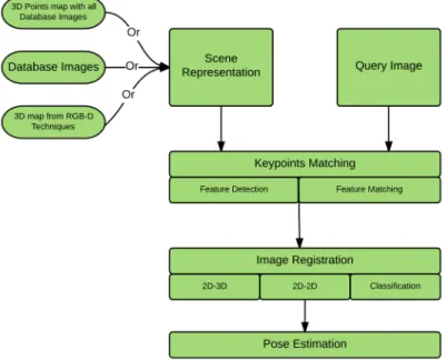
IBL can be solved using one of two approaches, namely 2D-3D matching or 2D-2D matching. 2D-3D matching consists of matching 2D features from a query image to a 3D point cloud map of the environment. The 3D map can be extracted either using Structure from Motion (SfM) techniques [62, 55, 56, 65, 59], or via RGB-D techniques [16, 49, 37]. In the former case, the map consists of a set of 3D points, along with their corresponding feature descriptors. In the latter case, the map consists of a featureless 3D point cloud. Alternatively, 2D-2D matching consists of matching a query image to a group of keyframe images that represent the scene. Figure 2.1 illustrates the main components in IBL.

IBL solutions face several challenges that can affect their robustness, accuracy and speed. Firstly, feature matching is dependent on feature viewpoint invariance; otherwise it is suscepti-ble to false matches due to scale, blur, and illumination changes. Secondly, IBL is also prone to the curse of dimensionality when dealing with scenes where there are thousands, sometimes millions of 3D points and their associated descriptors. In such situations, finding the exact cor-respondences becomes challenging. In addition, repeated patterns and structures as well as re-flected surfaces can also compound the problem.

IBL relies on three main building blocks for its solution as shown in Figure 2.1: (1) Keypoint matching which involves extracting the features and descriptors, then matching them to get the correspondences (2) Image registration to remove the wrong matches returned from the previous step and to send the images with enough inliers to the next step and (3) Pose estimation where the query pose is estimated and refined.

(24)

Figure 2.1: Image-Based Localization Main Components

2.3

KeyPoint Matching

The first step of IBL consists of establishing correspondences between keypoints extracted from query images with features extracted from a database keyframe. First, features are detected inside an image and then they are matched.

2.3.1

Feature Extraction

A feature is a salient point inside an image. Its robustness depends on its invariance to changes in scale and orientation. Many different types of feature detectors are available in the literature, with each one exhibiting different advantages and disadvantages. SIFT [30] has traditionally become the most popular feature detector; while it is somewhat robust to changes in viewpoint,

(25)

the computational overhead is very high. SURF [6] is another type of feature. SURF has a poor performance with changes in rotation when it is compared to SIFT which significantly influences the accuracy of the extracted feature points.The PCA-SIFT [23] proposes to reduce the computational overhead of SIFT by reducing its dimensionality; however, this comes at the cost of reduced accuracy and robustness. Affine SIFT [32] incorporated greater invariance to affine transformations, which showed more robust and accurate performances than the vanilla SIFT, but the feature extraction process takes a longer time. BRIEF [7] uses binary tests to classify trees. Their descriptor is a binary descriptor of 256 entries. It performs very poorly with changes in rotation, which restrict its use in IBL since it will affect the localization accuracy due to incorrect matches. ORB [43] is a fast binary descriptor based on BRIEF [7] and was introduced to solve the rotation problems with BRIEF. It performs better then regular BRIEF and faster then SIFT but still less accurately and less robustly than SIFT. FAST [42] uses a Harris corner filter and gives fast performance but suffers from sensitivity to orientation. This makes its use in IBL very specific to some scenes, mainly indoor scenes where the rotation effect is present. GPU-SIFT [54] is a parallel processing implementation of SIFT on GPU in real time to speed up the SIFT performance.

SIFT is most commonly used feature detector in IBL. It is mainly the most popular feature detector. Nevertheless, SIFT might not be the best accurate and robust feature detector method but this is not discussed in this thesis and is left for future work.

Once features are detected, one needs to recognize them from different viewpoints, and ac-cordingly, each image feature is associated with a description of its local neighbourhood, which is known as an image descriptor.

(26)

2.3.2

Feature Matching

Features are matched across frames by relying on their descriptors, which encode the image ap-pearance in the local neighbourhood of each feature. Finding the matches between descriptors is usually solved using linear search(or brute force) in IBL. The most obvious method for matching relies on brute force, where each image feature is compared to each feature descriptor in the database. Unfortunately, although effective, the process is very slow especially in large-scale scenes, where thousands or millions of 3D points have to be tested for a match.

Nearest Neighbour Search (NN) [14, 60] is the most common method used in IBL. Here, the search space is divided into subspaces of lower dimensions, thereby resulting in searching for matches in lower image scales. The disadvantage of such techniques is that the computational time grows exponentially when the size of the scene increases. To address its shortcoming known as Approximate Nearest Neighbour Search (ANN) [2, 4] attempts to find the neighbour that is most similar to the matched feature. Although it does not necessarily find the exact neighbour, it finds the most similar neighbour which in some cases might be the exact one.

To this date there are not any exact search methods that are faster then BF. All other methods like NN and ANN are optimization methods and are not considered exact. The main challenge of Image-based localization'is to find the correct matches. Thus the optimized methods used have to minimize the number of false matches while achieving fast computational times.

Fast Library of ANN (FLANN) [35] is a library of fast ANN methods to speed up the search in high dimensional spaces. These methods use either multiple randomized kd-trees or hierar-chical k-means trees:

(27)

1 Kd-trees [35] iteratively split the k-dimensional set of descriptors space. The data is split at each tree level at the value where the data scores the largest variance. This results in a hierarchy of splits called search trees. It tries to find the nearest neighbours by traversing all the leaves in the tree. Increasing the search space dimension requires a large amount of time to search all the leaves. An alternative more efficient approach proposed by [53] con-sists of visiting a reduced number of leaf nodes to find the approximate nearest neighbour. In the method known as the Forest of Randomized kd-trees [34], the split is chosen ran-domly among the ones featuring the largest variance. It increases the efficiency and gives similar accuracy to the kd-trees in approximating the nearest neighbour but at the cost of high memory requirements. The kd-trees method is the most common approach used in IBL [45] for matching. It presents the best compromise between accuracy and computa-tional time. Nevertheless, in larger environments where there are thousands or millions of descriptors, the matching speed of kd-trees decreases.

2 Hierarchical k-means trees [34] also known as a vocabulary trees [38] use k-means clus-tering to iteratively split the descriptors group into k clusters. The clusclus-tering stops when each cluster contains less then k descriptors. The approach traverses the tree to find the ap-proximate nearest neighbour corresponding to the closest cluster centre in each node. Due to its efficiency, hierarchical k-means is commonly used in IBL for matching descriptors. Nevertheless, it is subjected to miss correct correspondences due to quantization effects where a feature can get assigned to a cluster that does not contain many of its matches.

As an alternative to matching features, another approach is based on learning classes of fea-tures. Here, descriptors corresponding to the same feature are used to train a machine-learning

(28)

algorithm; then, any new feature is classified based on the attributed class of its descriptor. Donoser et al. [12] presented an alternative to the Approximate Nearest neighbour (ANN) by introducing a discriminative classification step called embedded random ferns. Their goal was to improve the feature matching by considering previous sightings of a specific feature as a class. This system scored a higher number of matches than tree-based but the quality of these matches remained questionable. The major shortcoming is the weakness of the classifier in global matching and its reliance on GPS tags to partition the search space into smaller regions. This approach will be further explained and discussed in Section 4.

2.4

Image Registration

The second building block of IBL is image registration, which is performed via 2D-3D corre-spondence, 2D-2D image matching, or classification.

2.4.1

2D-3D

The image registration step aims to find the correct matches (inliers) between a query image and a database of 3D points. . The standard approach to find the set of 2D-3D correspondences is by utilizing the tree-based approach(based on FLANN). To clarify this point, a number of features that are matched using the keypoint matching technique are not correct and using them would result in inaccurate localization. Therefore, it is necessary to follow the keypoint-matching step by image registration to help reduce the number of erroneous matches. To help remove false matches, one must perform what is known as the ratio test [30], where a match is only accepted

(29)

if the similarity between the distances to the first and second nearest neighbour is less then a certain threshold. Then RANSAC [40] is applied to remove the remaining outliers. RANSAC iteratively selects a random subset of all the matches, then uses this subset to estimate the camera transformation, and verifies the estimated transformation against all other matches. If the number of inliers after RANSAC applied is higher then 12 then the image can be considered registered and subsequently qualifies for pose estimation. Otherwise, it is discarded. The threshold of 12 inliers proposed by [29] is chosen to be high enough to make it unlikely for a false candidate to have this many inliers and low enough for true candidates with a low number of features not to be rejected.

The Tree-based approach (FLANN) is so slow when dealing with medium to large scale en-vironments because it performs the matching against the whole search space. During the past years, several improvements to image registration were proposed. Li et al. [28] presented a visi-bility graph(P2F), which sorts the 3D points in a map in terms of their visivisi-bility from the camera viewpoint corresponding to the different photos that were used to construct the map. Then, they used 3D-2D to guarantee that a sufficient number of inliers is found. Their algorithm stops after 100 correspondences are found. Then RANSAC is used to remove the outliers. Their local-ization results outperformed the tree-based approach in terms of speed but were less accurate. Li et al. [29] further improved the image registration by introducing co-occurrence RANSAC. This consists of a probabilistic model that uses a visibility model [29] to choose the highest set of 2D-3D matches that tends to co-occur using RANSAC. Then, they used 3D-2D checking to guarantee that a sufficient number of inliers were found. This approach slowed their previous approach but resulted in higher accuracy.

(30)

im-age registration. They clustered 3D points into bag-of-words and then sorted them based on a priority cost before matching them through a tree-based approach, stopping after one hundred matches were found. Their system is considerably faster then tree-based, P2F, and Co-occurrence RANSAC, but not as accurate as tree-based. Sattler et al. [46] improved their VPS system for registration by introducing active search, where the surroundings of a 2D-3D match are searched to find its nearest neighbours., This is followed by a 3D-2D matching to recover the matches from their VPS. Their system was faster then all the other approaches but lost some accuracy to VPS. All these registration approaches tackled city-scale scenes.

Shotton et al. [49] presented a different registration approach. They used a regression ran-dom forest method to train a featureless 3D map, reconstructed from RGB-D techniques. They matched the 2D points of a query image to their trained map to get the 2D-3D correspondences. Their method tackled small-scale environments and was faster, although less accurate than tree-based. Their work was not tested on city-scale sets and therefore cannot be easily compared to the previously mentioned registration approaches.

2.4.2

2D-2D

Although 2D-3D is more accurate and faster than 2D-2D in re-localization applications, image registration is performed using 2D-2D techniques to save computational time needed for fast localization. The scene is represented by a database of keyframes that cover that environment. 2D-2D image registration consists of assigning to each query image the corresponding keyframe that is most similar. Then, the set of 2D-2D correspondences between the matched images is computed. Similar to the 2D-3D matching, these matches are subjected to the ratio test [30] and

(31)

RANSAC [40] in order to remove the outliers. Again, if a sufficient number of inliers are found, the image is considered registered and the image qualifies for pose estimation.

In the work of Shotton et al. [16], an efficient encoding of each keyframe is performed by training their internal 2D pixels using random ferns and then matching each keyframe to the query image. The keyframes with the smallest distance to the query are then used to perform a 2D-2D match and thereby guarantee robust image registration. Their system performed better (in terms of accuracy and speed) at re-localization when a query image was close to a keyframe.

2.4.3

Classification

In addition to the more common 2D-3D, and 2D-2D image registration techniques, classification techniques can also be used to improve image registration. It is notable that although classifi-cation can be used as an alternative to the above techniques, it can also be used with 2D-3D or 2D-2D to further improve the registration.

In classification techniques, Heisterklaus et al. [19] images are binned into multiple views using global descriptors. Then synthetic camera poses are created to cover all the remaining spaces in the environment; this is needed to ensure more robust correspondences in less time. Their system showed promising registration improvements.

2.5

Pose Estimation

Any image in which a sufficient number of features are matched and subsequently image regis-tration is successful can be used for estimating the camera pose (translation and rotation).

(32)

Cal-culating the camera pose of a camera depends on the underlying matching that was performed (i.e., 2D-3D or 2D-2D).

In the case of 2D-3D matching, the n-point perspective (pnp) method is used. It starts by computing the location of the 3D map points in the local frame of the camera. Then, the cam-era pose is estimated by calculating a rigid geometric transformation between the position of the points in the local frame and their position in the global frame. The computation of the transformation between local and global frames requires information about the intrinsic camera parameters. This information can be either known or unknown. In the case of known intrinsic parameters (mainly focal length and distortions), the rigid transformation is estimated from three 2D-3D matches and is referred to as three-point perspective pose problem (p3p). P3P defines the pose by aligning local and global point positions and yields up to 4 solutions. Kneip et al. [25] presents a very efficient solution to IBL using p3p. The six-point perspective pose problem (p6p) is widely used to compute the transformation in the case of unknown intrinsic parameters. It computes a full projection camera matrix including the focal length estimation from six 2D-3D matches and yields a single solution. Recently, Sattler et al. [47] presented a new method to estimate the transformation by using p3p while sampling the focal length. They achieved same accuracy as standard PnP with much faster speed. It is used to avoid evaluating all the solutions returned from PnP. Iterative pnp can optionally be used to refine the estimated camera pose.

In the case of the 2D-2D correspondence case, the camera pose is estimated using the funda-mental matrix of the camera. The method consists of estimating the camera fundafunda-mental matrix from a set of points using the epipolar geometry constraint between two cameras in the case of unknown intrinsic parameters. In the case of a calibrated camera (known intrinsic parameters), the 5-point algorithm estimates the projection matrix, here called essential matrix, from at least

(33)

5 2D-2D matches. The pose is usually then refined by using non linear error minimization tech-niques. In IBL, Levenberg-Marquardt (LM) [15], Gauss-Newton [44] and M-estimators [20] are the refinement approaches commonly used.

2.6

Summary

This chapter presented a literature review about IBL; The history of IBL was presented. Then the IBL problem was described and its three main stages (Keypoints matching, image registration and pose estimation) were presented. Each stage was fully described and the main works done in each stage were presented. These main approaches appear to have many shortcomings in terms of accuracy and computational performance mainly in search space reduction, clustering, feature matching and the quality of the solution is not consistent across all query images. The main approaches will be studied and the main shortcomings of each will be revealed in Chapter 4 to prove that IBL problem is not yet solved. In the next chapter, the focus will be on choosing the best software to reconstruct the 3D map of the environment.

(34)

Chapter 3

Creating The Scene Representation

3.1

Introduction

In this modern era, cameras are found everywhere. They are relatively cheap, light, and produce high-resolution images. These factors, along with the advances in Computer Vision, make a camera the sensor of choice for producing 3D models of any environment. Applications range from aerial mapping to mapping of indoor and outdoor land scenes, to mapping of underwater environments. Both filter-based techniques (Visual Simultaneous Localization and Mapping or Visual SLAM) [57, 11] and non-filtering methods (e.g., Structure From Motion or SFM) [31, 33, 24, 65] produce maps by concurrently localizing the position of the camera in the map. While all types of localization and mapping produce maps during localization, the quality of the maps differs based on the specifics of each implementation. The majority of real time localization applications tend to build the maps on the fly. This poses limitations that are still unsolved using

(35)

a monocular camera. There are many notable limitations. First, obtaining an accurate real world scale that is crucial for many applications like Augmented Reality(AR) is very hard with the use of a single monocular camera. Second, the computational time and memory requirements related to the platform that these applications are run on limit the algorithm use and can pose some constraints on the map and the environment size. For instance, PTAM [24] was mainly built for indoor AR applications and PTAMM [8] was built for mobile platforms with limitations on the size of the maps. The memory of the phone can deal with sparse maps with a limited number of features. Third, the built map quality is affected by the time and memory complexity which affects the robustness of the tracking. There are lots of applications that do not require the maps to be built on the fly. Having a good sparse 3D map which is used only for tracking can solve the above limitations concerning the IBL problem.

Building a sparse map with the least amount of points which clearly describes the scene using a single cheap camera has been evolving for several years now. The most notable, successful approaches were based on SFM and the best known approaches are currently Bundler [55, 56, 62] and VSFM [65, 64]. The evolution of Bundler in 2008 allowed IBL to start focusing on real-time applications using a 3D map in any environment. In this chapter, three different 3D modeling packages based on SFM are tested: VSFM [63], Bundler [62] and PTAM [24]. The objective is to assess the mapping ability of each of the techniques and choose the best one to use for reconstructing the IBL 3D map.

(36)

3.2

Packages Description

In this section we describe the basic functionality steps behind each of the packages. We will present the main methods used to do the 3D reconstruction so that we can differentiate between each package and understand the reasons behind the different results that will be shown later.

3.2.1

Bundler

The latest version of Bundler was released in 2010. This software aims to demonstrate the success of SFM techniques on unorganized images sets that may be found on the Web. The package uses a robust modified SFM approach to reconstruct 3D scenes out of these unordered images. The main methods upon which Bundler works are described below [55]:

A) Feature matching: Bundler uses the SIFT feature detector. Then, each pair of images is matched to get the Fundamental matrix. Here Bundler runs its own optimization to get a robust Fundamental matrix(F-matrix) using RANSAC as follows:

1) Compute a candidate F-Matrix for each RANSAC iteration using the eight point algo-rithm.

2) Run non-linear refinement of it.

3) Remove the outlier matches and get the recovered F-matrix.

4) Check if the number of remaining matches is less then 20, then remove all the matches. B) Modified SFM: Bundler organizes the matches into a connected set of matched keypoints across multiple images called a ’track’. The modified SFM approach is summarized below:

(37)

1) Bundler initializes cameras using pose estimation to avoid getting stuck in bad local minima. This is done by adding multiple cameras at a time.

2) Bundler uses different approaches to choose the initial 2 images. It chooses the pair of images that have the largest number of matched features and then estimates the camera parameters of this pair.

3) Bundler starts to add multiple cameras to the optimization. It begins by adding the cam-era with the greatest number of matches (whose 3D position has been already estimated) then follows that by adding any camera that has 0.75 of the total number of matches. 4) For each added camera, Bundler initialize the extrinsic and intrinsic parameters using Direct Linear Transformation (DLT). It also reads EXIF tags of the image where they take the focal length and compare it to the estimated one from DLT to initialize it.

5) For each added camera, Bundler adds tracks observed by that camera. Each track is added if it was observed by at least one recovered camera.

6) Bundler uses sparse BA to minimize the reprojection error at each iteration. After every run of the optimization, Bundler detects 3D outlier points that have high reprojection error in a track and then removes that track. Then optimization is rerun again until no outliers remain.

3.2.2

VisualSFM

The latest version of VSFM was released in 2013. The main target of this package was to reach a linear time incremental SFM. Wu in his paper [64] explains the major improvements that his

(38)

software presented to build a better 3D reconstruction. Basically, VSFM improved the SFM algorithm done in Bundler. The main methods upon which this software work are described below:

1) VSFM uses a new feature matching approach called "Preemptive Feature Matching". This method consists of: a) Sorting the SIFT features of each image in a decreasing scale order, b) Generating the frame pairs to be either fully matched or by taking a subset of images to be matched, c) Looping over each image pair by first choosing a number hcorresponding to the firsthfeatures to be matched. Then, it is essential to check if the number of matches is less than a certain threshold, then repeat the matching, and if it is not then do regular matching and geometry estimations.

2) VSFM uses multicore bundle adjustment [65] where the aim of BA is to refine the 3D position of features and camera parameters by minimizing the non-linear reprojection error function. This method uses implicit multiplication of the known Hessian matrices and Schur complements by the use of the Jacobian matrix. In this way, the function is linearized at each iteration.

3) VSFM uses a modified version of incremental SFM from Bundler. First, the software starts to do full BA only when the size of a model is increased by a certain threshold ratio due to the large amounts of cameras being added. But to reduce the error accumulation, VSFM always runs local partial/local BA on a certain number of recent frames. Second, point filtering is done on the 3D points that had large reprojection errors.

(39)

failed feature matches. This is done to recover these points and to have more features in the scene. Here the reprojection error threshold is increased to reach that goal. Then a full BA and point filtering is run again to improve the reconstruction and reduce the errors.

Thus, VSFM is characterized by the preemptive feature matching, multicore BA and incre-mental SFM that uses a mix of BAs and RT to maintain the accuracy of the 3D reconstruction.

3.2.3

PTAM

PTAM was released in 2007. Many updates were made on it and the latest was PTAMM (parallel tracking and multiple mapping) in 2011. The main approach is described in [24] and [8]. It splits the tracking and mapping into 2 parallel threads. The main approach is described below:

A) Mapping is the main part that we are interested in when dealing with 3D scene recon-struction. The main difference from other SFM softwares is that they only update the map based on a keyframe. In other words, they have their own way to add frames to the mapping thread. The main algorithm works as follows:

1) PTAM uses stereo initialization: They take the first 2 keyframes, run FAST-10 features extraction, match the 2 images to get the F-matrix, use RANSAC to remove outliers, recal-culate F-matrix using inliers, optimize for getting the correct Essential matrix and finally triangulate the 3D points.

2) Adding Keyframes: PTAM only adds a frame, which becomes a keyframe, to continue constructing the map based on satisfying the following 3 conditions: a) if tracking quality

(40)

is good, b) if a minimum of 20 frames has passed since the last keyframe was added and c) if the camera has moved a minimum distance from the last keyframe pose.

3) 3D points are added to the map by feature matching along epipolar lines between the latest keyframe added to the map and its closest keyframe in terms of camera position using triangulation.

4) BA: LM algorithm is used to refine the camera positions and 3D triangulated points. When a new keyframe is added, BA is interrupted.

B) Tracking is run parallel to the mapping thread. The main steps are summarized below: 1) At each frame grabbed by the camera, the image is converted to grayscale. Then a 4 level pyramid is created for each frame. Fast-10 feature detector is run at each level. 2) A predicted camera pose is estimated using a decaying velocity model.

3) 3D map points are projected into the image according to the frame predicted pose in point 2 using a calibrated pin hole camera model.

4) 50 3D points are projected at coarse level into the image plane and searched for. Given successful patch matches between the new image and its closest keyframe, the camera pose is updated by minimizing an objective function that accounts for the reprojection error. Then 1000 points are projected at a fine level and the same procedure is repeated to refine the updated pose.

(41)

3.3

Results

3.3.1

Datasets and Testing Methodology

Three datasets composed of hundreds of images taken by our camera (point grey as raw data, logitech as png). Each dataset is described below:

1. Jbeil Roman Theatre:

Images of a very old Roman Theatre located in Byblos-Jbeil were taken by a non-calibrated Logitech camera. The images were taken as Keyframes inside PTAM where 31 keyframes were stored for testing for this scene as input images to other packages to ensure having a fair comparison.

2. University of Waterloo Robotics Group Lab:

2000 Images for a well dense lab located at the University of Waterloo were taken as raw data from an uncalibrated Point Grey Camera. The best 400 frames out of the 2000 were chosen to reconstruct this scene. The aim was to show the camera effect of the reconstruction by taking the images as raw uncompressed data.

3. University of Waterloo Engineering 5 Building:

400 Images for a symmetrical shaped building were taken as raw data from our Point Grey uncalibrated camera to be the input images to the packages. This building was chosen due to its symmetrical shape effect on the reconstruction along with its reflection effects caused by the glass

(42)

The three packages were used as blackboxes where some parameters were tuned to have a fair comparison. In VSFM, we changed the maximum feature matching number, and it was tuned so that more features can be matched. The minimum and maximum reprojection error thresholds were tuned by trial and error and we set the best ones equally for the three packages. In Bundler, the camera initialization thresholds were tuned. In PTAM, the number of minimum keyframes was lowered along with the minimum distance threshold from the camera to get more keyframes, since the goal is to tackle the mapping thread of PTAM.

3.3.2

Results

This section will present the reconstructed 3D maps scenes for each dataset used along with their corresponding reprojection errors.

Roman Theater Dataset The reconstructed 3D sparse maps for Jbeil Roman theater are shown in Fig. 3.1. Fig. 3.1a and 3.1b show a side and a front view of the resultant sparse map of the theater from VSFM respectively. Fig 3.1c and 3.1d also show a side and a front view for the map reconstructed from PTAM respectively. Fig. 3.1e show the Bundler reconstructed map. It is clear that the reconstruction from VSFM and PTAM was good and it clearly shows the layout of the theater, with a fair advantage to VSFM where it shows a more robust structure of the monument. In contrast, the Bundler reconstruction was poor and did not even reflect the theater aspect.

The reprojection error in pixels associated with the reconstructed maps from Bundler and VSFM are shown in Fig. 3.2. Fig. 3.2 shows that the error coming from VSFM is a bit higher than the one coming from Bundler. The total average reprojection error for VSFM was 3.09

(43)

whereas it scored 2.47 for Bundler. The main reason why Bundler had a lower error than VSFM is simply because of the number of 3D features. The sparse map from VSFM had 8661 features whereas PTAM’s map had 7100 and Bundler’s map had only 3246. So Bundler’s reprojection error was lower than the VSFM reprojection error because it was computed on 2.8 times less number of features. The number of features also reflects the fact that VSFM and PTAM returned good maps with a fair advantage to VSFM’s map.

(44)

(a) Jbeil map from VSFM side view

(b) Jbeil map from VSFM front view

(c) Jbeil map from PTAM side view

(d) Jbeil map from PTAM front view

(e) Jbeil map from Bundler

(45)

Figure 3.2: Reprojection error Vs feature ID associated with the reconstructed maps for Jbeil Roman Theatre

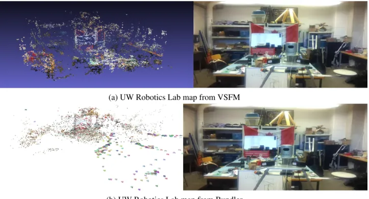
University of Waterloo Robotics Group Lab Dataset The reconstructed 3D sparse maps for the University of Waterloo Robotics Lab are shown in Fig. 3.3. Fig. 3.3a shows the resultant sparse map of the lab from VSFM. Fig. 3.3b shows the Bundler reconstructed map. This time, Bundler showed an acceptable reconstruction where the lab can be identified. But compared to VSFM the Bundler results become marginally bad since VSFM showed again a really good 3D sparse map. In Fig. 3.3a we can clearly see that VSFM maintained the lab structure and main components and a person can clearly identify some of the lab components such as the Canadian

(46)

(a) UW Robotics Lab map from VSFM

(b) UW Robotics Lab map from Bundler

Figure 3.3: Reconstructed 3D sparse maps for UW Robotics Lab

flag.

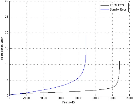
The reprojection error in pixels associated with the reconstructed maps from Bundler and VSFM are shown in Fig. 3.4. The figure shows that the error coming from VSFM is lower than the one coming from Bundler. The total average reprojection error for VSFM was 1.35 whereas it scored 3.01 for Bundler. The sparse map from VSFM had 12881 features whereas Bundler’s map had 8962. Those numbers reflect the sparsity of the map and the fact that VSFM again returned the best map. Alternatively, Bundler this time was able to get an acceptable number of features to build its map.

(47)

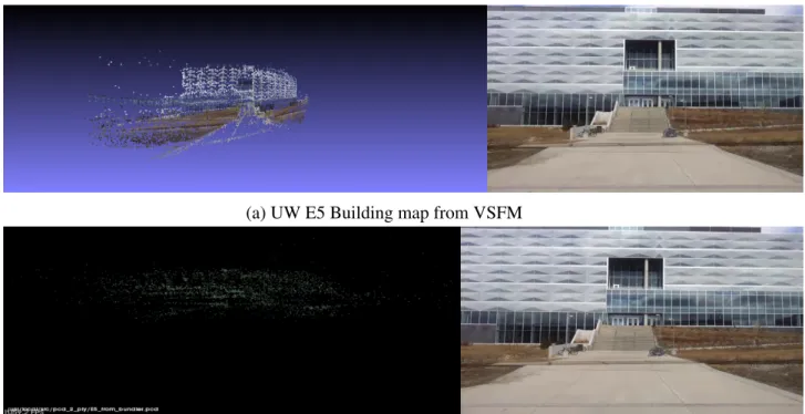
University of Waterloo Engineering 5 Building Dataset The reconstructed 3D sparse maps for the University of Waterloo’s Engineering 5 Building are shown in Fig. 3.5. Fig. 3.5a shows the resultant sparse map of the lab from VSFM. Fig. 3.5b shows the Bundler reconstructed map. Again VSFM showed a good reconstruction where the E5 building structure was clearly visible. Although the map was visually good, we must note that it was returned in 2D plane and not in 3D plane. This is due to the symmetrical shape and the lighting reflections coming from the glass of that building. In contrast, the Bundler reconstruction was pretty poor and did not even reflect

Figure 3.4: Reprojection error Vs feature ID associated with the reconstructed maps for UW Robotics Lab

(48)

the building aspect.

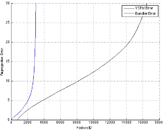
The reprojection error in pixels associated with the reconstructed maps from Bundler and VSFM are shown in Fig. 3.6. The figure shows that the error coming from VSFM is more then 2 times higher than the one coming from Bundler. The total average reprojection error for VSFM was 13.24 whereas it scored 5.44 for Bundler. Those numbers show that the VSFM reconstructed map is indeed a decent one, but there is something wrong in the 2D reprojections. The sparse map from VSFM has 16478 features, while Bundler’s map had only 2994. So Bundler’s reprojection error was lower than the VSFM reprojection error because it was computed on 5.5 times less number of features. The number of features also demonstrates the fact that VSFM is again the best package.

(49)

(a) UW E5 Building map from VSFM

(b) UW E5 Building map from Bundler

(50)

Figure 3.6: Reprojection error Vs feature ID associated with the reconstructed maps for UW E5 building

(51)

3.4

Analysis and Discussion

In this section, the analysis of the results is discussed and the shortcomings of each tested package are revealed, along with their effect on IBL.

First, VSFM'’s robust and accurate mixing of Re-triangulation (RT) and BA is a major reason it produced the best sparse maps. Reconstruction shows that the RT step is handling the drifting errors where some features marked as outliers were re-optimized using RT. a Many of them were found to be inliers and were refined using BA. This gave VSFM a main advantage over PTAM and Bundler since t PTAM and Bundler only run optimization and do not re-triangulate the outliers.

Second, it was noticed that VSFM’s multicore BA gave their optimization of the camera parameters and features positions more accuracy over Bundler and PTAM. Bundler used only regular global BA when they had to add multiple cameras to the optimization to save time. -Thus, their BA estimations returned lots of outliers. PTAM, on the other hand, used a mixed global and local BA which gave their maps a large number of inliers and helped to reduce the accumulation error.

Third, image matching which is the bottleneck of SFM, SLAM and IBL plays the major role in favour of VSFM. VSFM’s preemptive feature matching approach gave VSFM a high number of robust matches relative to PTAM and Bundler. This method offers a very low computational cost and allows one to focus efforts on the features that are most likely to be matched. This, combined with the mixing of RT and BA, allowed a large number of inliers, and so a large number of features in the reconstructed map. This is a major necessity for IBL since good quality matches in the map lead to more inliers and better localization accuracy. Bundler'’s major

(52)

problem causing poor results was its own image matching. It is summarized by the numbers of cameras registered for the reconstruction. A very large number of cameras failed to initialize, leaving the reconstruction with a small amount of registered cameras (for example only 328 images out of the 400 were registered for the E5 Building dataset). This affected the number of features, thus the complete reconstruction. It is mainly caused by two major things. First, the images could not be matched because they belong to a part of the scene which might be disconnected from each other. In addition, there was excessive blur and noise, and little overlap with other images. This results in a very few number of matches, where Bundler set a threshold of 20 remaining matches in order to register the camera. Second, Bundler uses a prior pose estimation to initialize the camera to avoid getting stuck in local minima. W This failed in l many cases and marked the images as bad ones, and therefore did not initialize them. The poor quality of matches that Bumdler returns will give less localization accuracy.

Fourth, Bundler used a camera model that does not handle the lens distortion, which causes large reconstruction errors. This is why in Bundler’s maps there exist a lot of reconstructed features that should be marked as outliers.

Fifth, it was noticed that PTAM sometimes inserted wrong features into the map with high errors. This happened when tracking quality was poor.

Finally, some chosen environments might be challenging to reconstruct, especially those who have symmetrical or repeating structures or do not have strong features like the E5 Building dataset. Even VSFM had problems reconstructing such scenes.

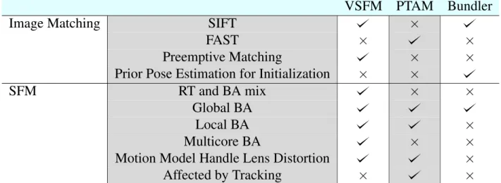
To summarize, all of these main algorithmic differences explained above are tabulated in Table 3.1. It is crucial for IBL to choose the software that provides the best quality of points, i.e.

(53)

VSFM

PTAM

Bundler

Image Matching

SIFT

×

FAST

×

Preemptive Matching

×

Prior Pose Estimation for Initialization

×

SFM

RT and BA mix

×

Global BA

Local BA

×

Multicore BA

×

Motion Model Handle Lens Distortion

×

Affected by Tracking

×

Table 3.1: Main algorithmic differences for each package.

the largest number of correct 3D points. For this reason, VSFM was chosen to reconstruct the 3D maps for IBL.

(54)

Chapter 4

IBL State of the Art Evaluation

1

In this chapter the state of the art in IBL techniques will be described. Also, the different datasets used in IBL will be discussed. The methodology that was followed to ensure a fair comparison is also presented. Then, the results of the study on each of the available approaches will be presented. This will be followed with a comparison utilizing the results taken from the papers describing closed-source systems. Finally, the results will be analyzed and discussed by present-ing the shortcompresent-ings and strengths of each approach.

4.1

Main Approaches Description

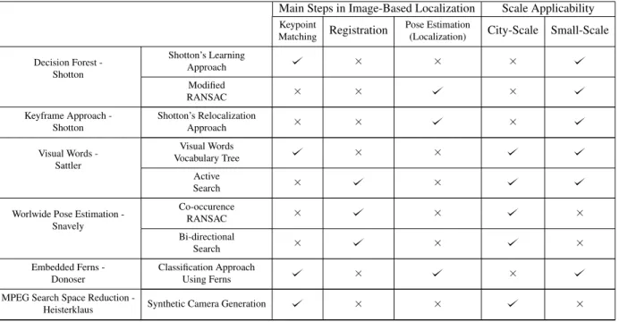
In this section the state of the art in IBL techniques are presented. Table 4.1 lists six different systems taken from the literature, along with the advantages and disadvantages of each system.

1_{The contents of this chapter will be submitted to the Robotics and Automation Magazine, 2016 IEEE.}

Co-authors include: Charbel Azzi, John Zelek, Daniel Asmar and Adel Fakih. I hereby verify that I will be the principal author. The material will be paraphrased.

(55)

Table 4.1: This table shows the area of contributions for each major approach in the main steps of IBL and its scalability application

Main Steps in Image-Based Localization Scale Applicability Keypoint

Matching Registration

Pose Estimation

(Localization) City-Scale Small-Scale Decision Forest -Shotton Shotton’s Learning Approach × × × Modified RANSAC × × × Keyframe Approach -Shotton Shotton’s Relocalization Approach × × × Visual Words -Sattler Visual Words Vocabulary Tree × × Active Search × ×

Worlwide Pose Estimation -Snavely Co-occurence RANSAC × × × Bi-directional Search × × × Embedded Ferns -Donoser Classification Approach Using Ferns × ×

MPEG Search Space Reduction

-Heisterklaus Synthetic Camera Generation × × ×

IBL techniques are typically designed for two different types of scale; namely, (1) small indoor scales, which consist of hundreds of images and result in tens of thousands of 3D points and (2) a large city-scale, in which the representative database contains thousands of images and millions of 3D points. Some of these selected techniques are open-source in nature and they are the most commonly referred to. The list includes the decision forest [49], the Keyframe approach [16], Visual Words [46], Worldwide Pose Estimation [28], Embedded Ferns [12] and MPEG search space reduction [19].

(56)

4.1.1

Decision Forest

Shotton et al. [50] presented an IBL system that focused on improving the Keypoints matching and pose estimation steps. Their main contributions were: (1) their regression forest to represent the scene and (2) their modified RANSAC for pose estimation.

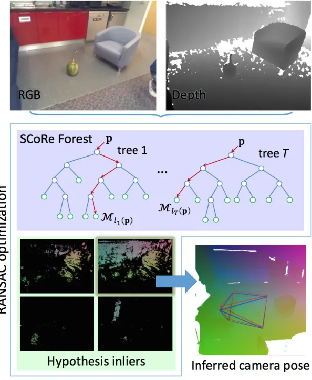
Their main technique is illustrated in Figure 4.1 They used an RBD-D sensor to get both RGB images and their corresponding depth. The images have known poses computed from the RGB-D technique [49, 16, 37]. They determined the pixel location of each image and used this position to train a regression forest [1, 27, 51]. The depth and camera poses are used to compute the 3D scene coordinates by training the forest at every image pixel. The forest is mainly used to generate a mathematical representation of the scene from the input database images from which the output will be the 3D position of each pixel point. This will result in a featureless 3D map. The pixels of a query image are matched to the 3D map points through the regression forest. Then a modified version of Preemptive RANSAC based on energy minimization is used to remove the outliers. If more then 12 inliers are found, the image is registered and its pose is estimated and optimized.

4.1.2

Keyframe Approach

Shotton et al. [16] presented a keyframe approach for re-localization application. Their main idea focuses on finding the closest keyframe to the query image to correct the current pose estimation using a new simplified random ferns [39] approach.

(57)

keyframe in the database intomequal pixel locations. Thus each image is divided into m ferns and each fern is divided into 4 nodes to represent the intensity of each pixel (RGB and Depth). They encode each fern in the image by doing a simple binary test. A query image is taken and divided to m equal locations and compared respectively to all the keyframes in the database using the trained ferns. Then, the block hamming distance (BlockHD) between the query image and each keyframe is computed from the resulting binary test. The hamming distance is a number that denotes the difference between two binary blocks and the blockHD counts the number of differing blocks. The closest keyframes with the smallest distance to the image are chosen and matched via standard FLANN in order to obtain the 2D-2D correspondences. If more then 12 inliers are found after RANSAC, than the image is registered and its pose is estimated.

4.1.3

ACG Localizer

Sattler et al. [46, 45] presented a complete IBL system that aimed to reduce the search space problem when dealing with large city-scale environments. They improved the keypoint match-ing step by their Vocabulary Prioritized Search (VPS) [45] algorithm, described in the previous section, and their active search method improved the image registration step. They used a 3D point cloud map where they presented their VPS, illustrated in Figure 4.2, to cluster the 3D points into bag-of-words and form a vocabulary tree. Each point is stored by the mean of all its SIFT descriptors [30]. The tree is sorted based on a priorities strategy that takes into account the co-visibility of each 3D point in the database image. Then, they start their active search algorithm, illustrated in Figure 4.3 by performing a standard FLANN 2D-3D matching between the query image descriptors and the 3D point in the vocabulary tree until one hundred matches are found.

(58)

There is a high probability that the nearest neighbours of a matched 3D point will have matches in the query image. Thus, the neighbours of each matched 3D point undergo a 3D-2D matching with 2D features in the query image. The outliers are then removed via RANSAC and if more then 12 inliers are found, the image is registered.

4.1.4

Worldwide Pose Estimation

Snavely et al. [28] address the image registration step in IBL and propose an improvement based on their co-occurrence RANSAC and bi-directional contributions. They worked on a city-scale mapping of the environments. Their work consists of performing a standard FLANN 2D-3D between the query features and all the 3D maps until one hundred matches are found. Co-occurrence RANSAC is then applied on those matched. It consists of dividing the resultant matches into subsets. Then they use a probabilistic model to return the subsets with the highest probability. These subsets are the starting set that RANSAC will begin with to remove the outliers. If more then 12 inliers are found, then the query is registered and qualifies for pose estimation. Otherwise, the matches undergo a bi-directional search, which consists of performing a 3D-2D matching to guarantee that a sufficient number of inliers is found.

4.1.5

Embedded Ferns

Donoser et al. [12] presented a new keypoints matching technique that can be used for IBL. Their main contribution was presenting a new classification technique called embedded ferns.

(59)

FLANN to get the 2D-3D by a discriminative classification step called embedded random ferns. They basically used all the descriptors representing each 3D point to train a classifier, then used random ferns based on the projections. They only stored the classifier and removed the images and descriptors to save memory. They required a GPS prior on camera position to restrict the classification into certain areas of the scene from which the query image is taken.

4.1.6

MPEG Search Space Reduction

Heisterklaus et al. [19] improved the keypoints matching and image registration steps. Their main idea is to reduce the search space in large city-scale environments by presenting synthetic views to cover the space for faster 2D-3D matching.

For each keyframe in the database, they extract the MPEG Compact Descriptors for Visual Search descriptor (CDVS) [13]. Each one consists of a global descriptor and compressed lo-cal descriptors. A CDVS test model is used to generate a compact model of the real and the synthetic camera views within an image based on frustum culling. Thus, for each keyframe, its corresponding three hundred most relevant features and its global descriptor are stored to form the compact 3D model. The three hundred most relevant SIFT descriptors are extracted from a query image along with its CDVS descriptor. These 300 descriptors are matched via 2D-2D with the 3D model to get a score for match. Then the 2D-3D correspondences are computed from the highest scored matched 2D-2D. If enough inliers are found after RANSAC, then the image is registered and its pose is estimated.

(60)

(61)

Figure 4.2: Vocabulary-based Prioritized Search(VPS). (Sattler et al., 2011)

(62)

4.2

Datasets and Methodology

Table 4.2 presents the eight datasets used for the assessment of IBL systems. The first six datasets are large and represent some major cities in the world. The sets were reconstructed using Bundler [62] from images that are available on the web.

The query images are the test images against which the approaches are validated. The table shows the number of 3D points that each map consists of. Dubrovnik [29], Rome [29], Quad and Vienna [22] datasets consist of a few million 3D points reconstructed from images taken by Flickr users. The Aachen [46] dataset also has a few millions 3D points and the query images were taken by Flickr users via telephone over a two year period. This makes them more difficult to process than the previous three datasets due to geometrical defection and changes that could have happened during two years. Landmark 1k [28] is the most popular 1k landmark on Flickr and together with San Francisco [28], they are considered the largest datasets, featuring tens of million of 3D points. Microsoft researcher introduced the 7 scene Dataset [50] which consists of images for seven different indoor scenes taken using an RGB-D Kinect.

Table 4.2: The major datasets used in IBL along with the total number of database images, query images and 3D points.

Dataset Total # of Images # of Query Images # of 3D points [Million]

Dubrovnik [29] 6044 800 1.9 Rome [29] 15179 1000 4.1 Vienna [22] 1324 266 1.1 Quad [10] 6514 348 1 Aachen [46] 3047 369 1.5 Landmarks 1k [28] 204000 1000 38 San Francisco [28] 610000 803 30