University of Pennsylvania
ScholarlyCommons
Publicly Accessible Penn Dissertations
1-1-2014
Approximate Inference for Determinantal Point
Processes
Jennifer Ann Gillenwater
University of Pennsylvania, [email protected]
Follow this and additional works at:http://repository.upenn.edu/edissertations
Part of theComputer Sciences Commons,Engineering Commons, and theStatistics and Probability Commons
This paper is posted at ScholarlyCommons.http://repository.upenn.edu/edissertations/1285
Recommended Citation
Gillenwater, Jennifer Ann, "Approximate Inference for Determinantal Point Processes" (2014).Publicly Accessible Penn Dissertations. 1285.
Approximate Inference for Determinantal Point Processes
Abstract
In this thesis we explore a probabilistic model that is well-suited to a variety of subset selection tasks: the determinantal point process (DPP). DPPs were originally developed in the physics community to describe the repulsive interactions of fermions. More recently, they have been applied to machine learning problems such as search diversification and document summarization, which can be cast as subset selection tasks. A challenge, however, is scaling such DPP-based methods to the size of the datasets of interest to this
community, and developing approximations for DPP inference tasks whose exact computation is prohibitively expensive.
A DPP defines a probability distribution over all subsets of a ground set of items. Consider the inference tasks common to probabilistic models, which include normalizing, marginalizing, conditioning, sampling,
estimating the mode, and maximizing likelihood. For DPPs, exactly computing the quantities necessary for the first four of these tasks requires time cubic in the number of items or features of the items. In this thesis, we propose a means of making these four tasks tractable even in the realm where the number of itemsandthe number of features is large. Specifically, we analyze the impact of randomly projecting the features down to a lower-dimensional space and show that the variational distance between the resulting DPP and the original is bounded. In addition to expanding the circumstances in which these first four tasks are tractable, we also tackle the other two tasks, the first of which is known to be NP-hard (with no PTAS) and the second of which is conjectured to be NP-hard. For mode estimation, we build on submodular maximization techniques to develop an algorithm with a multiplicative approximation guarantee. For likelihood maximization, we exploit the generative process associated with DPP sampling to derive an expectation-maximization (EM) algorithm. We experimentally verify the practicality of all the techniques that we develop, testing them on applications such as news and research summarization, political candidate comparison, and product recommendation.
Degree Type
Dissertation
Degree Name
Doctor of Philosophy (PhD)
Graduate Group
Computer and Information Science
First Advisor
Ben Taskar
Second Advisor
Keywords
determinantal point processes, expectation-maximization, learning, MAP inference, random projections, submodular maximization
Subject Categories
APPROXIMATE INFERENCE FOR
DETERMINANTAL POINT PROCESSES
Jennifer Gillenwater
A DISSERTATION in
Computer and Information Science
Presented to the Faculties of the University of Pennsylvania in Partial Fulfillment of the Requirements for the
Degree of Doctor of Philosophy
2014
Ben Taskar, Associate Professor of Computer and Information Science Supervisor of Dissertation
Emily Fox, Adjunct Professor of Computer and Information Science Co-Supervisor of Dissertation
Lyle Ungar, Professor of Computer and Information Science Graduate Group Chairperson
Dissertation Committee:
Michael Kearns, Professor of Computer and Information Science Ali Jadbabaie, Professor of Electrical and Systems Engineering Alexander Rakhlin, Assistant Professor of Statistics
APPROXIMATE INFERENCE FOR
DETERMINANTAL POINT PROCESSES
COPYRIGHT
2014
Jennifer Gillenwater
Licensed under a Creative Commons Attribution-ShareAlike 4.0 License.
To view a copy of this license, visit:
Acknowledgments
ABSTRACT
APPROXIMATE INFERENCE FOR DETERMINANTAL POINT PROCESSES
Jennifer Gillenwater Ben Taskar
Emily Fox
In this thesis we explore a probabilistic model that is well-suited to a variety of subset selection tasks: the determinantal point process (DPP). DPPs were origi-nally developed in the physics community to describe the repulsive interactions of fermions. More recently, they have been applied to machine learning problems such as search diversification and document summarization, which can be cast as subset selection tasks. A challenge, however, is scaling such DPP-based methods to the size of the datasets of interest to this community, and developing approximations for DPP inference tasks whose exact computation is prohibitively expensive.
Contents
Acknowledgements iii
Abstract iv
List of Tables ix
List of Figures xi
List of Algorithms xii
1 Introduction 1
1.1 Motivating subset selection applications . . . 2
1.2 Expressing set-goodness as a determinant . . . 5
1.3 Definition of a DPP . . . 7
1.4 Motivating DPP inference tasks . . . 8
1.5 Thesis contributions . . . 10
2 DPP Basics 12 2.1 Geometric interpretation . . . 12
2.2 Inference . . . 14
2.2.2 Marginalizing . . . 16
2.2.3 Conditioning . . . 17
2.2.4 Sampling . . . 21
2.2.5 MAP estimation . . . 26
2.2.6 Likelihood maximization . . . 27
2.2.7 Maximizing entropy . . . 29
2.2.8 Computing expectations . . . 29
2.3 Closure . . . 31
2.4 Dual representation . . . 32
2.4.1 Normalizing . . . 33
2.4.2 Marginalizing . . . 33
2.4.3 Conditioning . . . 33
2.4.4 Sampling . . . 34
2.5 Quality-similarity decomposition . . . 36
3 DPP Variants 37 3.1 Cardinality-constrained DPPs . . . 37
3.2 Structured DPPs . . . 40
3.3 Markov DPPs . . . 42
3.4 Continuous DPPs . . . 44
4 Dimensionality Reduction 46 4.1 Random projections . . . 47
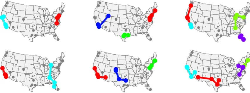
4.2 Threadingk-SDPPs . . . 50
4.3 Toy example: geographical paths . . . 52
4.4 Threading document collections . . . 54
4.4.1 Related work . . . 56
4.4.2 Setup . . . 57
4.4.3 Academic citation data . . . 59
4.4.4 News articles . . . 59
4.5 Related random projections work . . . 68
4.6 Related DPP work . . . 69
4.6.2 Nyström approximation . . . 74
5 MAP estimation 81 5.1 Definition of submodularity . . . 83
5.2 Log-submodularity of det . . . 84
5.3 Submodular maximization . . . 86
5.3.1 Monotonef . . . 86
5.3.2 Non-monotonef . . . 88
5.3.3 Constrainedf . . . 90
5.4 Polytope constraints . . . 91
5.5 Softmax extension . . . 92
5.5.1 Softmax maximization algorithms. . . 97
5.5.2 Softmax approximation bound . . . 98
5.5.3 Rounding . . . 101
5.6 Experiments . . . 104
5.6.1 Synthetic data . . . 104
5.6.2 Political candidate comparison . . . 106
5.7 Model combination . . . 108
6 Likelihood maximization 109 6.1 Alternatives to maximizing likelihood . . . 110
6.2 Feature representation . . . 113
6.3 Concave likelihood-based objectives . . . 114
6.4 Non-concave likelihood-based objectives . . . 117
6.5 MCMC approach for parametric kernels . . . 118
6.6 EM approach for unrestricted kernels . . . 120
6.6.1 Projected gradient ascent . . . 120
6.6.2 Eigendecomposing . . . 122
6.6.3 Lower bounding the objective . . . 123
6.6.4 E-step . . . 124
6.6.5 M-step eigenvalue updates . . . 126
6.6.6 M-step eigenvector updates . . . 127
6.7.1 Baby registry tests . . . 132 6.7.2 Exponentiated gradient . . . 137
7 Conclusion 139
List of Tables
2.1 Complexity of inference. . . 15
2.2 Kernel conditioning formulas. . . 19
4.1 News timelines automatic evaluation . . . 66
4.2 News timelines Mechanical Turk evaluation . . . 66
4.3 News timeline runtimes . . . 67
6.1 Baby registry dataset sizes . . . 132
List of Figures
1.1 DPP product recommendations . . . 2
1.2 Geometry of determinants . . . 6
1.3 Sampling/MAP for points in the plane . . . 10
2.1 DPP sampling algorithms . . . 23
3.1 Example structured DPP sample . . . 40
4.1 Geographical path samples . . . 52
4.2 Fidelity of random projections . . . 53
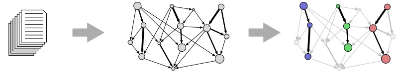
4.3 Document threading framework . . . 54
4.4 Random projection of a single vector . . . 55
4.5 Cora citation threads . . . 60
4.6 News graph visualization . . . 62
4.7 k-SDPP news timelines . . . 63
4.8 DTM news timelines . . . 64
4.9 News timeline Mechanical Turk task . . . 67
5.1 Det log-submodularity in 2-3 dimensions . . . 84
5.2 Symmetric greedy algorithms . . . 90
5.4 Softmax upper-bounding multilinear . . . 95
5.5 Concave softmax cross-sections . . . 99
5.6 Synthetic MAP results. . . 105
5.7 Political candidate comparison results . . . 107
6.1 Kernel learning algorithms . . . 122
6.2 Baby registry EM evaluation . . . 134
6.3 EM product recommendations . . . 136
List of Algorithms
1 O(N k3)DPP Sampling . . . . 23
2 O(N k2)DPP Sampling . . . . 23
3 Dual DPP Sampling. . . 35
4 Nyström-based Dual DPP Sampling . . . 79
5 greedy for DPP MAP . . . 86
6 randomized-symmetric-greedy for DPP MAP . . . 90
7 symmetric-greedy for DPP MAP . . . 90
8 cond-grad (Frank-Wolfe) . . . 98
9 softmax-opt for DPP MAP . . . 98
10 constrained-greedy for DPP MAP . . . 107
11 Projected gradient for DPP learning . . . 122
1
Introduction
When there is a mismatch between the quantity of a resource available and con-sumer capacity, mechanisms for selecting a subset of the overlarge group are often invoked. For example: for a limited number of job openings, there may be an exces-sive number of applicants, or, for a camping expedition, there may be more supplies available than a camper can fit in his backpack. Moreover, as the amount of in-formation readily available to us via electronic resources grows, we are increasingly facing this type of dilemma in the setting where the overlarge group is a form of information. For this reason, summarization mechanisms are becoming more and more important for paring information down to manageable portions that human (and machine) learners can easily digest. Subset selection is one elementary way of formalizing the summarization task.
majors, so as to have a variety of informed perspectives on the company’s projects. The ability to balance the dual goals of quality and diversity is at the core of most effective subset selection methods.
1.1
Motivating subset selection applications
To give additional insight into situations where such subsets are desired, we list here examples of how common applications are typically cast in the subset selection mold:
• Product recommendation(McSherry, 2002; Gillenwater, Kulesza, Fox, and Taskar, 2014): For retailers with a large inventory, selecting a good subset of products to recommend to a given customer is important not only for boosting revenue, but also for saving the customer time. In this setting, a good subset should contain products that other customers have rated highly, but should also exhibit diversity—if a customer already has a carseat in their cart, they most likely will not buy an additional carseat, no matter how popular it is with other consumers. Figure1.1 illustrates the type of product diversity that a determinantal point process (DPP) can achieve.
Graco Sweet Slumber Sound Machine
VTech Comm.
Audio Monitor Boppy Noggin Nest
Head Support
Cloud b Twilight Constellation Night Light
Braun ThermoScan Lens Filters
Britax EZ-Cling Sun Shades
TL Care Organic Cotton Mittens
Regalo Easy Step Walk Thru Gate
Aquatopia Bath Thermometer Alarm
Infant Optics
Video Monitor
Figure 1.1: A set of10baby safety products selected using a DPP.
• Document summarization (Lin and Bilmes, 2012; Kulesza and Taskar,
content of the documents. There are many variations on this task, including some where the ground set consists of N structures, rather than just simple
sentences; see for example the news threading application in Chapter4.
• Web search(Kulesza and Taskar,2011a): Given a large number of images or documents, consider the problem of selecting a subset that are relevant to a user query. Note that diversity is important in this setting as many queries are ambiguous (e.g. the search “jaguars” could refer to the cats, the cars, or the football team).
• Social network marketing (Hartline, Mirrokni, and Sundararajan, 2008): Consider a social network consisting ofN people. Suppose a seller has a digital good that costs nothing to copy (unlimited supply). In this setting, a common marketing strategy is “influence-and-exploit”: give the product to a subset of the people for free, then offer it to the rest of the network at a price. Intu-itively, the people who get the product for free should be high-degree nodes in the network, but also spread out such that no one will be too many hops from a product owner.
• Auction revenue maximization (Dughmi, Roughgarden, and Sundararajan,
2009): Given a base set of bidders, a pool ofN potential bidders, and a budget
k, a common task is to recruit a subset ofk additional bidders for the auction. This is sometimes called the “market expansion problem”.
• Sensor placement for Gaussian Processes (Krause, Singh, and Guestrin,
2008): Suppose there are N possible locations for sensors (e.g. for measuring pressure, temperature, or pollution). For a given sensor budget, at most k
sensors can be placed. Thus, it is important to be able to select a subset of the possible locations at which to actually place sensors, such that the measure-ments from these sensors will be as informative as possible about the space as a whole.
“sky” and “earth” is a common task, with k = 2). The segmentation task can be formulated as the problem of identifying one pixel (or superpixel) to serve as the “center” for each segment. Thus, the segmentation task reduces to selecting a size-k subset of an image’sN pixels.
• Pose tracking(Kulesza and Taskar,2010): Consider the problem of identify-ing the pixels correspondidentify-ing to each person in a video. For each video frame, a subset of the pixels must be chosen. Diversity is important in this setting because people tend to occupy disjoint locations in space, so the goodness of a subset tends to increase as its spatial diversity within a given frame increases.
• Network routing (Lee, Modiano, and Lee, 2010): Given the graph of a net-work, suppose that each link (edge) has some failure probability. Consider the problem of selecting a set of k paths from a source node to a target node such that if a message is sent along all of these paths, failure to deliver (at least one copy of ) the message to the target is minimized. The best set of paths will be high-quality (all links on paths will have low failure probability), but also diverse (the failure of a link on one path should not hurt the other paths).
• Motion summarization (Affandi, Kulesza, Fox, and Taskar, 2013b): Given videos consisting of individuals performing a specific activity, consider the task of selecting a subset of the N video frames to summarize the activity. For example, the main motions involved in an activity such as basketball can be summarized by a few frames that are diverse in terms of the position of an athlete’s limbs.
There are also several basic machine learning tasks that are sometimes cast as subset selection problems:
• Clustering (Elhamifar, Sapiro, and Vidal, 2012; Reichart and Korhonen,
2013;Shah and Ghahramani,2013;Kang,2013): GivenN data points, select a subset ofkpoints to serve as cluster centers or as representatives of the overall
dataset.
The complexity of the tasks mentioned in this section is increased by the frequent practical need for constraints on the selected subset, Y ⊆ {1, . . . , N}. These range
from relatively simple cardinality constraints (|Y| ≤k, |Y| =k), to intersections of multiple matroids. See Chapter5for additional discussion of subset constraints.
1.2
Expressing set-goodness as a determinant
Having established some motivation for solving subset selection problems where the end goal is a high-quality but diverse set, in this section we consider basic measures of quality and diversity that lead directly to the definition of a determinantal point process (DPP).
Given N items, let item ibe represented by aD-dimensional feature vectorBi ∈
RD×1. For example, in the case of document summarization each sentence is an item,
andDmight be the size of the vocabulary. Each entry inBi could be a count of the
number of occurrences of the corresponding vocabulary word, normalized in some reasonable manner. One simple way to interpretBi is to assume that its magnitude,
∥Bi∥2, represents the quality of item i, and that its dot product with another item’s
feature vector,Bi⊤Bj, corresponds to the similarity between these two items.
For sets of size 1, the goodness of a set can then reasonably be represented by the quality of its only item, or any monotonic transformation of that quality. For example, we could score each singleton set{i}according to its quality squared,∥Bi∥22.
In geometric terms, this is the squared length (1-dimensional volume) of Bi. It is
also (trivially) the determinant of the1×1matrixBi⊤Bi.
As a measure of how good a set consisting of two items is, it is desirable to have an expression that not only rewards high quality, but also penalizes similarity. Ex-tending the geometric intuition from the singleton setting, for {i, j} the squared area (2-dimensional volume) of the parallelogram spanned byBi andBj would be
a reasonable choice. See Figure 1.2 for an example. Theorem 1.1 establishes that the expression for this squared area is: ∥Bi∥22∥Bj∥22 −(Bi⊤Bj)2. The first term here
is the product of the items’ squared qualities and the second term is the square of their similarity, so it is clear that this expression captures our stated goal of rewarding quality while penalizing similarity.
feature space
quality =pB>
i Bi
similarity =B>
i Bj
Bi+Bj
Bi
Bj pro
j?
BiB
j
Tuesday, August 5, 14
Figure 1.2: The area of the parallelogram outlined byBi andBj corresponds to the
square root of the proposed set-goodness measure. Left: Reducing ∥Bj∥2
corre-sponds to reducing the quality of item j, hence making the set {i, j}less desirable. Notice that the reduction in item quality produces a reduction in parallelogram area.
Right: Reducing the angle betweenBi andBj corresponds to making the items less
diverse, again making the set{i, j}less desirable. The parallelogram area is similarly
reduced in this case.
Bi, Bj, andBi+Bj is √
∥Bi∥22∥Bj∥22−(Bi⊤Bj)2.
Proof. See Section2.1.
In addition to being related to area, this set-goodness formula can be expressed as a determinant:
det
(
∥Bi∥22 Bi⊤Bj
Bi⊤Bj ∥Bj∥22
)
=det
([
Bi⊤
Bj⊤
]
[Bi Bj] )
=∥Bi∥22∥Bj∥22−(Bi⊤Bj)2. (1.1)
The geometric and determinantal formulas for size-1 and size-2 sets extend in a fairly straightforward manner to sets of all sizes. Consider replacing length and area withk-dimensional volume. For a set of size 3, this is the canonical notion of volume. For larger sets, applying the standard “height × base” formula gives the recursive definition:
vol(B) = ∥B1∥2vol
(
proj⊥B1(B2:N) )
where proj⊥B
1(·) projects to the subspace perpendicular to B1, and the subscript
B2:N indexes all columns of B between2and N, inclusive. Theorem1.2establishes
that the square of this geometric formula is equal to the natural extension of Equa-tion (1.1), the determinantal formula, to larger size sets: det(B⊤B) =vol(B)2.
Theorem 1.2. Given a D×N matrix B with N ≤ D, consider the N-parallelotope whose vertices are linear combinations of the N columns of B with weights in {0,1}:
V = {α1B1 +. . .+αNBN | αi ∈ {0,1} ∀i ∈ {1, . . . , N}}. The volume of this N
-parallelotope is√det(B⊤B).
Proof. See Section2.1.
This basic extension of a natural set-goodness measure from size-1 and size-2 sets to sets of arbitrary size brings us immediately to the definition of a determinantal point process (DPP).
1.3
Definition of a DPP
The previous section informally defined a set-goodness score in terms of a feature matrixB. Here we give a more rigorous definition.
At a high level, stochastic processes are generalizations of random vectors. Dis-crete, finite stochastic processes are equivalent to random vectors: a sequence of
N random variables [Y1, . . . , YN], associated with a joint probability distribution
P(Y1 =y1, . . . , YN = yN). A discrete, finite point process is a type of discrete, finite
stochastic process where each variable is binary,yi ∈ {0,1}, indicating the occurrence
or non-occurrence of some event (e.g. neuron spike, lightening strike, inclusion of a sentence in a summary). This thesis focuses on discrete, finite determinantal point processes (DPPs), which are point processes where the occurrence of one event cor-responds with a decrease in the probability of similar events. That is, these processes exhibit repulsion between points, resulting in diversity.
Formally, let the points (sometimes referred to as events or items) under consid-eration be those in the set Y = {1,2, . . . , N}. Let 2Y refer to the set of all subsets ofY, which has magnitude 2N. This includes the empty set, ∅, and the full set,Y.
We will frequently use Y ⊆ Y to denote one of these subsets, and Y to denote a
(2005), a random variable Y drawn according to a (discrete, finite) determinantal point processPLhas value Y with probability:
PL(Y =Y)∝det(LY), (1.3)
for some positive semi-definite (PSD) matrix L ∈ RN×N. The L
Y here denotes the
restriction ofL to rows and columns indexed by elements ofY: LY ≡ [Lij]i,j∈Y. It
is assumed that det(L∅) = 1. In what follows, we will use the shorthand PL(Y) for
PL(Y =Y)where the meaning is clear.
Note that the definition given by Equation (1.3) is similar to the geometrically motivated set-goodness score from Section 1.2, but withL in place ofB⊤B. These definitions are in fact equivalent. To see this, note thatB⊤Bcan be any Gram matrix. The equivalence of the definitions then follows immediately from the equivalence of the class of Gram matrices and the class of PSD matrices: every PSD matrix can be written as the Gram matrix from some set of (potentially infinite dimensional) vectors, and every Gram matrix is PSD.
1.4
Motivating DPP inference tasks
Having established the formal definition of a DPP, it is now possible to discuss its associated inference problems and how each relates to the subset selection task. Common inference operations include MAP estimation, sampling, marginalizing, conditioning, likelihood maximization, and normalizing.
• MAP estimation: Finding the mode, or as it is sometimes referred to in con-ditional models, maximum a posteriori (MAP) estimation, is the problem of finding the highest-scoring set. This is the set for which the balanced mea-sure of quality and diversity developed in Section 1.2 is highest. Clearly, this is the inference operation we would ultimately like to perform for the subset selection tasks from Section 1.1. Unfortunately, this problem corresponds to volume maximization, which is known to be NP-hard. Thus, for the problem of selecting the highest-scoring set under a DPP, we must rely on approxima-tion algorithms.
com-bining DPPs with other probabilistic models to build novel generative stories. Sampling is also one very simple way of approximating a DPP’s mode; since higher-quality, more diverse sets have greater probability mass, we are more likely to sample them. Even this simple MAP approximation technique can often yield better sets than non-DPP-based subset selection methods.
• Marginalizing: Sampling algorithms, as well as several other MAP estimation techniques, rely on the computation of marginal probabilities for efficiency. More concretely, one of the first steps in a basic DPP sampling algorithm is to estimate the marginal probability for each individual item i ∈ Y. The first item for the sample set is then selected with probability proportional to these marginals.
• Conditioning: As with marginalization, being able to condition on the inclu-sion of an item i ∈ Y is important to the efficiency of sampling algorithms. Independent of its use in sampling though, conditioning can easily be seen to have practical importance. Recall for a moment the product recommendation application from Section 1.1, and suppose that we are presented with a cus-tomer who already has several items in their cart. To recommend additional items, it makes sense to condition on the items already selected.
• Likelihood maximization: For some subset selection tasks appropriately-weighted feature vectors are readily available and can be used to form a feature matrixB, from which we can compute a DPP kernel L=B⊤B. However, in
most cases it is not known up front how important each feature is. Instead, we often have access to indirect evidence of feature importance, in the form of examples of “good” subsets. Leveraging this information to learn feature weights, or to infer the entries of the kernel matrixLdirectly, can be done by maximizing the likelihood of the “good” subsets. The result is a kernel that can be used to find good subsets for related subset selection tasks.
• Normalizing: Being able to compute set goodness scores that all fall into the
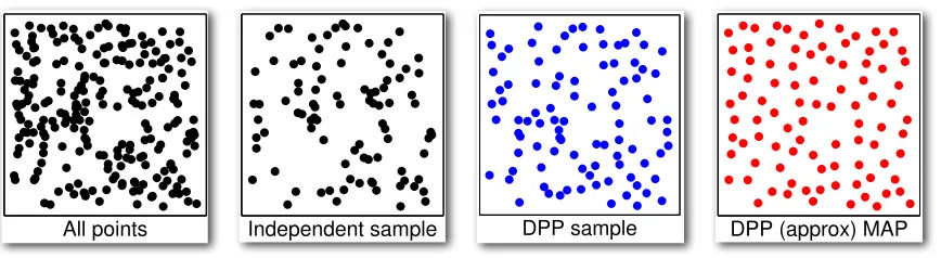
All points Independent sample DPP sample DPP (approx) MAP
Monday, August 4, 14
Figure 1.3: From left to right: A ground set ofN points; sampling each point inde-pendently with probability1
2; sampling from a DPP with a Gaussian kernel; applying
a DPP MAP approximation algorithm. The DPP sample exhibits greater diversity than the independent sample, but the DPP MAP approximation is the most diverse.
1.5
Thesis contributions
DPPs can typically be efficiently normalized, marginalized, conditioned, and sam-pled. Table 2.1 in the next chapter gives the exact time complexities, but roughly these operations require time cubic in the number of items, N, or features, D, of these items: O(min(N3, D3))time. Unfortunately, there are some practical settings
where cubic time is too expensive. For example, recall the document summarization task from Section1.1. If the documents we wish to summarize consist of all the New York Times articles from the past year, then the number of sentences N will be in the millions. Moreover, if we use the vocabulary of these articles as the feature set, then the number of featuresDwill be (at least) in the tens of thousands. Exact nor-malization, marginalization, conditioning, and sampling algorithms cannot handle data of this size. Thus, in this thesis we explore approximations for the setting where bothN andDare large.
be NP-hard. This means that to learn a DPP that puts as much weight as possible on observed “good” subsets, we must rely on local optimization techniques.
In this thesis, we seek to better address all three of these hard problems: the
large-N, large-D setting, MAP estimation, and likelihood maximization. It might seem easier to skirt these issues by switching to a simpler model than the DPP—clearly, given all of the references in Section 1.1, there are many non-DPP-based subset selection methods to choose from. However, experimental results, such as those in Sections4.4.4,5.6, and6.7, suggest that sticking with the DPP paradigm is often the better choice. The primary contributions of this document are summarized below.
• Chapter 2: We review the basic properties and representations of DPPs. For the core inference tasks, we survey algorithms and hardness results.
• Chapter3: We discuss several useful DPP variants: k-DPPs, structured DPPs, Markov DPPs, and continuous DPPs. Several of these variants are relevant to the results in later chapters.
• Chapter4: We analyze the impact of randomly projecting features down to a lower-dimensional space and establish a bound on the difference between the resulting DPP and the original. We illustrate the practicality of the projected DPP by applying it to select sets of document threads in large news and research collections.
• Chapter 5: We build on submodular maximization techniques to develop an algorithm for finding the DPP MAP problem with a multiplicative 1
4
-approximation guarantee. We validate the proposed algorithm on a political candidate comparison task.
• Chapter6: We derive an expectation-maximization (EM) algorithm for learn-ing the DPP kernel, motivated by the generative process that gives rise to DPP sampling algorithms. We show its superiority relative to projected gradient ascent on a product recommendation task.
2
DPP Basics
This chapter discusses the basic properties, algorithms, identities, and hardness re-sults associated with DPPs. For additional background, references to mathemat-ical surveys, the use of DPPs as models in physics (e.g. for fermions), theoretmathemat-ical point processes that are determinantal (e.g. edges in random spanning trees, non-intersecting random walks), proofs of many of the theorems stated in this section, and a list of related point processes (e.g. Poisson, hyperdeterminantal), see Kulesza
(2012).
2.1
Geometric interpretation
Section 1.2 described the connection between determinants and volumes of par-allelotopes. To sharpen those intuitions, in this section we provide proofs for the associated theorems. First, for the case of the2×2 determinant, then for the more generalN ×N case.
Proof. (Of Theorem1.1.) This is a straightforward application of the “base×height” formula for the area of a parallelogram. LetBi serve as the base. Then:
where proj⊥B
i(·)projects to the subspace perpendicular toBi. Using the Pythagorean
theorem to re-write this projection:
∥proj⊥Bi(Bj)∥22+∥proj∥Bi(Bj)∥ 2
2 =∥Bj∥22 (2.2)
∥proj⊥Bi(Bj)∥2 =
√
∥Bj∥22− ∥proj∥Bi(Bj)∥ 2
2. (2.3)
Now, consider the basis formed by the vectors constituting the columns of a matrix
A. According to Meyer (2000, Equation 5.13.3), the matrix PA = A(A⊤A)−1A⊤
projects to the vector space spanned by those columns. Applying this withBi asA:
proj∥B
i(Bj) = Bi(B
⊤
i Bi)−1Bi⊤Bj =
BiBi⊤
∥Bi∥22
Bj. (2.4)
Combining Equations (2.3) and (2.4), and squaring the area:
area2 =∥B i∥22
(
∥Bj∥22−
BiBi⊤
∥Bi∥22
Bj 2 2 ) (2.5)
=∥Bi∥22∥Bj∥22−
∥Bi∥22
∥Bi∥42
∥BiBi⊤Bj∥22 (2.6)
=∥Bi∥22∥Bj∥22− 1
∥Bi∥22
∥Bi∥22(Bi⊤Bj)2 (2.7)
=∥Bi∥22∥Bj∥22−(Bi⊤Bj), (2.8)
where Equations (2.6) and (2.7) follow from the fact that norms are homogeneous functions, which means that scalars such as ∥Bi⊤Bi∥2 and Bi⊤Bj inside a norm are
equivalent to powers of these scalars outside the norm.
We now show the derivation of the more general determinant-volume relation-ship forN dimensions.
Proof. (Of Theorem 1.2.) We proceed by induction on N. For N = 1, volume
is length. The length ||B1||2 is trivially the square root of the 1× 1 determinant
det(B1⊤B1) = B1⊤B1. Now, assuming the theorem is true for N −1, we will show
that it holds forN.
Write BN = BN∥ +BN⊥, where B
∥
N is in the span of {B1, . . . , BN−1} and BN⊥ is
matrices, identity matrices with wi added to entry (i, N): Ti,N(wi) = I +1iwi1⊤N,
where1iindicates anN×1vector with zeros in all entries except for a one in theith.
Let B˜ be identical to B, but with BN replaced byBN⊥. We can relate B to B˜ via the
elementary transformation matrices: B = ˜BT1,N(w1). . . TN−1,N(wN−1). Taking the
determinant ofB⊤B, these transformations disappear; the determinant of a product decomposes into individual determinants, and the determinant of an elementary transformation matrix is 1. Thus, det(B⊤B) = det( ˜B⊤B)˜ . Writing out the new productB˜⊤B˜:
˜
B⊤B˜ =
(
B1:⊤N−1B1:N−1 B1:⊤N−1BN⊥
BN⊥⊤B1:N−1 B⊥N
⊤
BN⊥
)
. (2.9)
The orthogonality of BN⊥ means that B1:⊤N−1B⊥N is all zeros, as is BN⊥⊤B1:N−1. Thus
the determinant is:
det( ˜B⊤B˜) =det(B1:⊤N−1B1:N−1)BN⊥
⊤
BN⊥. (2.10)
By the inductive hypothesis, the first term here is the squared volume of the
(N − 1)-parallelotope defined by B1:N−1. Letting B1:N−1 serve as the base of the N-parallelotope defined by B, the height component of the “base × height” vol-ume formula is ||BN⊥||2. This is exactly the square root of the second term above,
BN⊥⊤BN⊥.
2.2
Inference
This section provides background on various common DPP inference tasks. The complexity of these tasks is summarized in Table2.1.
2.2.1 Normalizing
The definition of a DPP given in Equation (1.3) omits the proportionality constant necessary to compute the exact value ofPL(Y). Naïvely, this constant seems hard to
compute, as it is the sum over an exponential number of subsets: ∑Y′:Y′⊆Ydet(LY′).
Fortunately though, due to the multilinearity of the determinant, this sum is in fact equivalent to a single determinant: det(L+I). This is a special case of Theorem2.1
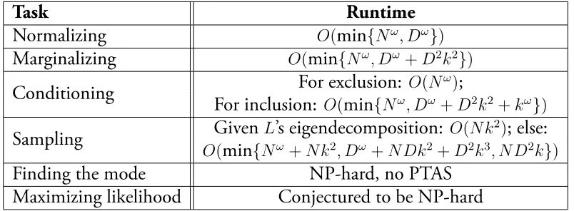
Task Runtime
Normalizing O(min{Nω, Dω})
Marginalizing O(min{Nω, Dω+D2k2})
Conditioning For exclusion: O(N
ω);
For inclusion: O(min{Nω, Dω+D2k2+kω})
Sampling Given L’s eigendecomposition: O(N k
2); else:
O(min{Nω+N k2, Dω+N Dk2+D2k3, N D2k})
Finding the mode NP-hard, no PTAS Maximizing likelihood Conjectured to be NP-hard
Table 2.1: Complexity of basic inference tasks. The size of the DPP’s ground set isN, andωdenotes the exponent of matrix multiplication. If each item in the ground set is associated with a feature vector (such as theBi of Section1.2), thenDdenotes the
vector’s length. We assumeD≤N. For marginalizing, conditioning, and sampling,
k is the size of the set marginalized, conditioned on, or sampled, respectively.
Theorem 2.1. For anyA⊆ Y:
∑
Y:A⊆Y⊆Y
det(LY) =det(L+IA), (2.11)
where IA is the diagonal matrix with ones in the diagonal positions corresponding to
elements ofA=Y \A, and zeros everywhere else.
Proof. SeeKulesza(2012, Theorem 2.1).
Typically, a single N ×N determinant for a PSD matrix is computed by
tak-ing the matrix’s Cholesky decomposition. This decomposition re-expresses a PSD matrix, such as Lor L+I, as the product of a triangular matrix and its transpose:
L+I =T T⊤. The determinant can then be computed as the square of the product ofT’s diagonal elements: ∑N
i=1T 2
ii. Naïve algorithms can compute the Cholesky
de-composition in 1 3N
3 operations (multiplications). More nuanced algorithms exhibit
improved performance for largeN. For example,Bunch and Hopcroft(1974) show
that the complexity of triangular factorization is identical to that of matrix mul-tiplication. Building on the Strassen matrix multiplication algorithm, they obtain Cholesky decompositions in time <2.45Nlog27 ≈2.45N2.807 (Bunch and Hopcroft,
the naïve approach for N ≈ 31,000 and above. While there are matrix multiplica-tion algorithms that are asymptotically faster than Strassen’s, these are not used in practice. For instance, the Coopersmith-Winograd algorithm has a complexity of
O(N2.375), but the big-O notation hides much too large of a constant coefficient for
this algorithm to be practical. In analyzing the complexity of algorithms presented in this thesis, we will useωto denote the exponent of whatever matrix multiplication algorithm is used. For practical purposes though, think ofωas roughly3.
2.2.2 Marginalizing
Just as the probability of a particular set, PL(Y = Y), is proportional to a
sub-determinant of a kernel L, the probability of the inclusion of a set, P(Y ⊆ Y), depends on the sub-determinant of a kernel closely related to L.
Theorem 2.2. For a DPP with kernelL, the matrixK defined by:
K =L(L+I)−1 =I−(L+I)−1 (2.12)
has minors satisfying:
P(Y ⊆Y) =det(KY). (2.13)
Proof. SeeKulesza(2012, Theorem 2.2).
We can also invert Equation (2.12) to expressLin terms of K:
L=K(I−K)−1 = (I−K)−1−I . (2.14)
We will refer to the matrixK as themarginal kernel. From Equation (2.13), two properties ofK are immediately obvious: first, since marginal probabilities must be non-negative, K must be PSD; second, since marginal probabilities must be < 1,
I −K must be PSD. An equivalent way of stating this second condition is to say
that K’s eigenvalues must be ≤ 1. Examining the eigendecomposition ofK and L
further clarifies their relationship. They share the same eigenvectors, andKsquashes
L’s eigenvalues down to the[0,1]range:
L=VΛV⊤=
N ∑
i=1
λiviv⊤i , K =
N ∑
i=1
λi
1 +λi
wherevi is the ith column of the eigenvector matrixV.
SinceK andLeach contain all of the information needed to identify a DPP, we
can use either one as the representation of a DPP. In fact, given K it is actually not even necessary to convert to L to obtain the probability of a particular subset. As shown byKulesza(2012, Section 3.5), we can write:
PL(Y =Y) = |det(K−IY)|. (2.16)
The redundancy ofKandLcomes with one caveat though: Ldoes not exist if any of
K’s eigenvalues are exactly1. This is clear from Equation (2.14), where the inverse is incomputable forK with an eigenvalue of1; an eigenvalue of1for K would imply an eigenvalue of∞forL. As will be made clear by the sampling algorithms though, as long as some non-zero probability is assigned to the empty set, K’s eigenvalues will be<1.
In terms of the complexity of converting between LandK, if this is done using Equations (2.12) and (2.14) then the dominating operation is the inversion. The naïve algorithm for matrix inversion runs in time2N3. Strassen’s matrix
multiplica-tion algorithm runs in time<4.7Nlog27(Bunch and Hopcroft,1974, Paragraph 2 of
the introduction) and can be used to compute a matrix inverse in time<6.84Nlog27
(Bunch and Hopcroft,1974, Final sentence of Section 4). This approach is more effi-cient than the naïve one forN ≈600and above. If instead we convert fromLtoKby computing an eigendecomposition, this tends to be slightly more expensive. While asymptotically (asN → ∞) it has the same complexity as matrix multiplication, the algorithms that achieve this complexity are not practical unlessN is extremely large. In practice, we instead rely on algorithms such as Lanczos to convert L or K to a
similar tridiagonal matrix, then apply divide-and-conquer algorithms such as those described in Gu and Eisenstat (1995) to compute the eigendecomposition of this matrix. (For real, symmetric matrices this is faster than relying onQR decomposi-tion algorithms.) The overall complexity for computing the eigendecomposidecomposi-tion of
LorK is then≈4N3.
2.2.3 Conditioning
that it is possible to write the resulting set probabilities as a DPP with some modified kernelL′ such thatPL′(Y =Y) =det(L′Y)/det(L′+I). Formulas for these modified
kernels are given in Table 2.2. We useLA to denote the kernel conditioned on the inclusion of the set A and L¬A to denote the kernel conditioned on the exclusion
of A. The (N − |A|)×(N − |A|) matrix LA is the restriction of L to the rows and columns indexed by elements in Y \A. The matrixIA is the diagonal matrix with ones in the diagonal entries indexed by elements ofY \Aand zeros everywhere else. The(N− |A|)× |A|matrix LA,A consists of the|A|rows and theA columns ofL.
For|A|=k, the complexity of computing these conditional kernels is:
• LA, KA: Equation (2.18) requires anN×N matrix inverse, which is anO(Nω)
operation. Equation (2.20) is dominated by its three-matrix product, an
O(N2k)operation. Formulas forKAhave the same complexity as theLAones.
• L¬A: Equation (2.19) simply requires copying(N −k)2 elements ofL.
• K¬A: Equation (2.22) requires an (N −k)×(N −k)matrix inverse, which is
anO((N −k)ω)operation.
The formulas in Table2.2can also be combined to produce kernels conditioned on both inclusion and exclusion. For instance, including the setAin and excluding
Aout the corresponding conditional kernel is:
LAin,¬Aout = ([LAout+IAin]Ain)−1−I . (2.17)
Equations (2.18) and (2.21) are derived in Kulesza (2012, Equation 2.42, 2.45). Equation (2.19) follows immediately from the definition of a DPP, and Equation (2.22) from the application of the L-to-K conversion formula of Equa-tion (2.12). We derive Equations (2.20) and (2.23) in Lemmas (2.4) and (2.5). These derivations rely upon the following identity.
Definition 2.3. Schur determinant identity: For a (p +q) ×(p +q) matrix M
decomposed into blocks A, B, C, D that are respectivelyp×p,p×q,q×p, andq×q:
M =
[
A B
C D
]
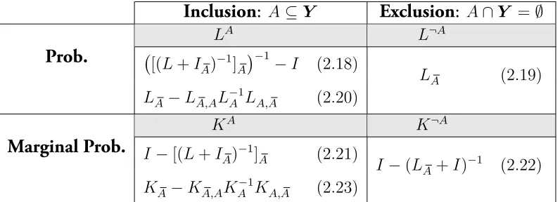
Inclusion: A⊆Y Exclusion: A∩Y =∅
Prob.
LA L¬A
(
[(L+IA)−1]A)−1−I (2.18)
LA (2.19)
LA−LA,AL−A1LA,A (2.20)
Marginal Prob.
KA K¬A
I−[(L+IA)−1]A (2.21)
I−(LA+I)−1 (2.22) KA−KA,AKA−1KA,A (2.23)
Table 2.2: Formulas for computing DPP kernels conditioned on the inclusion or exclusion of the setA⊆ Y.
the determinant ofM can be written in terms of the blocks:
det(M) = det(D)det(A−BD−1C). (2.25)
Given this identity, we can now derive Equations (2.20) and (2.23).
Lemma 2.4. For a DPP with kernelL, the conditional kernelLAwith minors satisfying:
P(Y =Y ∪A|A⊆Y) = det(L A Y)
det(LA+I) (2.26)
onY ⊆ Y \A, can be computed fromLby the rank-|A|update:
LA =LA−LA,AL−A1LA,A, (2.27)
assuming that the inverseL−A1 exists.
Proof. Conditioning on Ameans normalizing only by setsY′ that containA:
PL(Y =Y ∪A|A⊆Y) =
det(LY∪A) ∑
Y′:A⊆Y′⊆Y
det(LY′)
. (2.28)
Suppose, without loss of generality, that the items we are conditioning on are the last ones: A={N − |A|+ 1, . . . , N}. ThenLdecomposes into blocks:
L=
[
LA LA,A
LA,A LA
]
and by Schur’s identity we have that:
det(L) =det(LA)det (
LA−LA,AL−A1LA,A) . (2.30)
Let L′ denote the matrixLA−LA,AL−A1LA,A. Then applying Schur’s identity to the matrixLB∪A, whereB is any set such thatA∩B =∅, we have:
det(LB∪A) = det(LA)det (
LB−LB,AL−A1LA,B
)
=det(LA)det(L′B) . (2.31)
This allows us to simplify Equation (2.28). The numerator can be written:
det(LY∪A) =det(LA)det(L′Y). (2.32)
The normalizing term can similarly be simplified:
∑
Y′:A⊆Y′⊆Y
det(LY′) =
∑
Y′:A⊆Y′⊆Y
det(LA)det(L′Y′\A) (2.33)
= det(LA)
∑
Y′:A⊆Y′⊆Y
det(L′Y′\A) (2.34)
= det(LA) ∑
Y′:Y′⊆Y\A
det(L′Y′) (2.35)
= det(LA)det(L′ +I), (2.36)
where the final equality follows from Theorem 2.1. Plugging this back into Equa-tion (2.28):
PL(Y =Y ∪A|A⊆Y) =
det(LA)det(L′Y)
det(LA)det(L′+I)
= det(L
′
Y)
det(L′+I). (2.37)
Lemma 2.5. For a DPP with marginal kernelK, the conditional marginal kernelKA
with minors satisfying:
P(Y ⊆Y |A⊆Y) = det(KYA) (2.38)
onY ⊆ Y \A, can be computed fromK by the rank-|A|update:
KA=KA−KA,AKA−1KA,A, (2.39)
Proof. By the definition of conditional probability:
P(Y ⊆Y |A⊆Y) = P(Y ⊆Y, A⊆Y)
P(A⊆Y) =
det(KY∪A)
det(KA)
. (2.40)
Just as in Lemma 2.4, for any set B such that A∩B = ∅, application of Schur’s identity yields an expression for the determinant ofKB∪A:
det(KB∪A) = det(KA)det(KB′ ), (2.41)
whereK′ =KA−KA,AKA−1KA,A. This means that Equation (2.40) simplifies to:
P(Y ⊆Y |A⊆Y) = det(KA)det(K
′
Y)
det(KA)
=det(KY′ ). (2.42)
2.2.4 Sampling
Sampling algorithms to drawY ∼ PL rely on the eigendecomposition ofL(orK).
They are based on the fact that any DPP can be written as a mixture of elementary
DPPs, where the mixture weights are products ofL’s eigenvalues.
Definition 2.6. A DPP is elementary if its marginal kernel’s eigenvalues are all∈ {0,1}.
An elementary DPP is simpler than a general DPP in that it only places proba-bility mass on sets of a fixed size.
Lemma 2.7. Under an elementary DPP with k non-zero eigenvalues, the probability ofY =Y is zero for allY where |Y| ̸=k.
Proof. SeeKulesza(2012, Lemma 2.3).
Let V be a set of orthonormal vectors. LetVJ indicate selection of the columns
of V that correspond to the indices in a set J. We will write PVJ
to denote an elementary DPP with marginal kernelKVJ
:
KVJ = ∑
j:j∈J
vjv⊤j =V
J(VJ)⊤, PVJ
(Y ⊆Y) =det(KYVJ). (2.43)
Lemma 2.8. A DPP with kernel L that eigendecomposes as ∑N
i=1λiviv⊤i , is equal to
the following mixture of elementary DPPs:
PL(Y =Y) =
∑
J:J⊆{1,...,N}
PVJ
(Y =Y) ∏
j:j∈J
λj
1 +λj ∏
j:j∈/J (
1− λj
1 +λj )
. (2.44)
Proof. SeeKulesza(2012, Lemma 2.2) for a proof that:
PL(Y =Y) =
1
det(L+I)
∑
J:J⊆{1,...,N}
PVJ
(Y =Y) ∏
j:j∈J
λj. (2.45)
Rewriting det(L+I) =∏Ni=1(λi+ 1) and pushing this into theJ summation:
PL(Y =Y) =
∑
J:J⊆{1,...,N}
PVJ
(Y =Y) ∏
j:j∈J
λj
1 +λj ∏
j:j∈/J 1 1 +λj
. (2.46)
Since1− λj 1+λj =
1
1+λj, the result is obtained.
This mixture decomposition suggests a two-step sampling algorithm for DPPs. First, sample a subset of the eigenvectors,VJ, by including vectorj with probability
λj
1+λj. Second, sample a setY ⊆ Y according toP VJ
. Algorithm1, due to Hough, Krishnapur, Peres, and Virág(2006), fleshes out this two-step procedure. Assuming that the eigendecomposition ofLis given as input, then the most expensive part of the algorithm is in the second step, where we modify V such that it is orthogonal to the indicator vector eyi. This requires running the Gram-Schmidt process, an
O(N k2)operation. Overall, that makes Algorithm 1’s runtimeO(N k3).
It is possible to improve this runtime by avoiding the V updating. More
con-cretely, on each iteration we can lazily apply a simple conditioning formula to the diagonal of the elementary DPP’s marginal kernel. Algorithm 2 outlines this ap-proach. The first step, the selection ofJ, is the same as in Algorithm1. The second step only requires O(N k2) time though. To prove the correctness of Algorithm 2,
we rely on the following corollary and lemma.
Corollary 2.9. Given a marginal kernelK, the conditional marginal kernelK{i}, with
minors satisfyingP(Y ⊆Y |i∈Y) =det(KY{i}), can be computed fromK by the rank-1 update:
K{i} =K{i}− 1
Kii
Algorithm 1: O(N k3)DPP Sampling
1: Input: eigendecomp.VΛV⊤ ofL
2: J ← ∅
3: for j = 1, . . . , N do
4: J ←J∪ {j}with prob. λj 1+λj
5: V ←V:,J
6: Y ← ∅
7: while|Y|<|J|do
8: fori= 1, . . . , N do
9: zi ←
∑
v∈V v(i) 2
10: Selectyi withP r(yi) = zyi
|J|−|Y|
11: Y ←Y ∪ {yi}
12: j ←arg maxj′Vyi,j′
13: w←V:,j
14: V ←V:,{j}
15: V ←V − vj(1yi)wVyi,:
16: Gram-Schmidt(V)
17: Output: Y
Algorithm 2: O(N k2)DPP Sampling
1: Input: eigendecomp.VΛV⊤ ofL
2: J ← ∅
3: forj = 1, . . . , N do
4: J ←J ∪ {j}with prob. λj 1+λj
5: V ←V:,J
6: Y ← ∅
7: fori= 1, . . . , N do
8: zi ←
∑
v∈V v(i) 2
9: while|Y|<|J|do
10: Selectyi withP r(yi) = zyi
|J|−|Y|
11: Y ←Y ∪ {yi}
12: r|Y|←V Vy⊤i,:
13: for j = 1, . . . ,|Y| −1do
14: r|Y|←r|Y|−
rj(yi) rj(yj)rj
15: z ←z− z1
yir
2
|Y| 16: Output: Y
Figure 2.1: Two DPP sampling algorithms, both based on the elementary DPP decomposition of L. The slower algorithm computes an orthonormal basis for the subspaceV orthogonal toeyi for each point selected. The faster algorithm relies on
assumingKii̸= 0. The notationK{i},i indicates the vector composed of theith column of K, without its ith element.
Proof. This follows directly from Lemma2.5with A={i}.
Lemma 2.10. Let V ∈ RN×k be the eigenvectors of an elementary DPP’s marginal
kernel: K = V V⊤. Let Y ⊆ Y be size-k and arbitrarily order its elements [y1, . . . , yk].
UseYℓ to denote the subset{y1, . . . , yℓ}, withY0 =∅. Then we can express the(s, t)entry
of the conditional marginal kernel as follows:
KYℓ
st =Kst−
|Yℓ|
∑
j=1
KYj−1
syj K Yj−1
tyj
KYj−1
yjyj
, (2.48)
where KYℓ is the marginal kernel conditioned on the inclusion of Y ℓ.
Proof. We will proceed by induction on ℓ. For ℓ = 0 the statement of the lemma
reduces toKst∅ =Kst. This is trivially true, as the original marginal kernel is already
conditioned on the inclusion of the empty set. For the inductive step, we assume the lemma holds for ℓ − 1 and show that this implies it is also true for ℓ. From Corollary2.9we have the following expression forKYℓ:
KYℓ
st =K
Yℓ−1
st −
KYℓ−1
syℓ K Yℓ−1
tyℓ
KYℓ−1
yℓyℓ
. (2.49)
Moving theKYℓ−1
st term to the lefthand side yields:
KYℓ
st −K
Yℓ−1
st =−
KYℓ−1
syℓ K Yℓ−1
tyℓ
KYℓ−1
yℓyℓ
. (2.50)
The righthand side here is exactly the same as the difference between theℓandℓ−1
cases in the statement of the lemma.
We can now prove the correctness of Algorithm2.
Theorem 2.11. Given the eigendecomposition of a PSD matrix L = ∑Ni=1λiviv⊤i ,
Algorithm2 samplesY ∼ PL.
Proof. Lemma2.8 establishes that the mixture weight for elementary DPPPVJ
is:
∏
j:j∈J
λj
1 +λj ∏
j:j∈/J (
1− λj
1 +λj )
The first loop of Algorithm 2 selects VJ with exactly this probability. Thus, the
first loop of Algorithm 2 selects elementary DPPPVJ
with probability equal to its mixture component. Line 5 sets V = VJ, and all that remains to show is that the rest of the algorithm samplesY ∼ PV. In what follows, we will useK to refer to the
marginal kernel of the selected elementary DPP.
As in Lemma2.10, letYℓbe the set{y1, . . . , yℓ}. That is, the items selected during
the firstℓiterations of Line9’s while-loop. First, by induction on|Y|, we show that at Line15the variabler|Y|is equal toK
Y|Y|−1
:,y|Y| . In other words, we show thatr|Y|is the y|Y|th column of the marginal kernel conditioned on inclusion of {y1, . . . , y|Y|−1}.
For the base case,|Y| = 1, the result is immediate; Line12 sets r1 to K:,y1, and the
for-loop at Lines13 and14 does not change it. For the inductive case, |Y| =ℓ, we assumerj = K
Yj−1
:,yj for all j ≤ ℓ−1. Line 12sets rℓ = K:,yℓ and Line 13’s for-loop
updatesrℓexactly according to Equation (2.49) from Lemma2.10. Thus, at Line15
we have: rℓ=K Yℓ−1
:,yℓ , as desired.
Given this invariant onr|Y|, we now show that at Line10the variableziis always
equal to the marginal probability of selecting item i, conditioned on the current selection Y. That is, it is always the diagonal entry of the conditional marginal kernel: zi =KiiY. We again proceed by induction on |Y|. For the base case, Y =∅,
the marginal probability of an itemiisKii. Since Line8initializeszi =Vi,:Vi,⊤: =Kii,
the base case is trivially true. For the inductive case,|Y|=ℓ, the inductive hypothesis
says thatzi =K Yℓ−1
ii at Line10during theℓth execution of the while-loop. Then it is
clear that Line15 updateszi by applying Equation (2.49) for s =t. Thus, we have zi =KiiYℓ at Line10 during the next iteration of the while-loop, as desired.
Given this invariant on zi, all that remains to show is that the probability of
selecting elementito be theℓth item inY iszi/(k−ℓ+ 1), as in Line10. According
to Lemma2.7,Y must have|Y|=|J|at the end of the algorithm. Thus, whenℓ−1
items have been selected, there are stillk−ℓ+ 1ways in which itemicould be added to the final selection: it could be added as element ℓ, or ℓ+ 1, etc. Thus, Line 10
2.2.5 MAP estimation
Up to this point each of the inference tasks described—normalizing, marginalizing, conditioning, and sampling—can be performed in roughly O(N3) time. The task
of finding the MAP (or mode) of a DPP is more difficult. In fact, it is known to be NP-hard. This was shown byKo and Queyranne(1995), whose work focuses on the equivalent problem of selecting a subset of Gaussian random variables such that the entropy of the selected set is as large as possible. They start by assuming that the covariance matrixΣof the variables is known. Based onΣ, the entropy of any subset
Y of the variables can be computed according to:
H(Y) = 1
2ln
(
(2πe)|Y|det(ΣY) )
. (2.52)
For a fixed set size,|Y|=k, this is proportional to log det(ΣY). Ko and Queyranne
(1995) reduce the NP-complete “stable set” problem to the problem of maximizing log det(ΣY)subject to the cardinality constraint |Y| = k. Specifically, the stable set
problem asks: given anN-vertex graph Gand an integerk < N, decide whether G
contains a stable set withk vertices. A stable set is defined as a subsetS ofG’s nodes such that there are no edges between any of the nodes inS. The transformation of this graph problem into a determinant problem is accomplished by defining a PSD matrix based on the graph’s edges:
Σij =
3N ifi=j ,
1 if(i, j)is an edge inG ,
0 otherwise.
(2.53)
Ko and Queyranne (1995) show that finding a size-k minor of value greater than
(1−(3N)−2)(3N)k corresponds to finding a stable set of size k. Thus, the problem
of finding the largest size-k determinant of a PSD matrix is NP-hard, even if the matrix only has entries with values in {3N,1,0}. Ko and Queyranne (1995) ex-tend this reasoning to also show NP-hardness in the unconstrained setting, which is equivalent to the problem of finding the mode of a DPP with kernel Σ. They also
experiment with a branch-and-bound search algorithm for finding the best subset. It relies primarily on the eigenvalue interlacing property to define an upper bound.
Definition 2.12. Eigenvalue interlacing property: LetM be anN ×N symmetric
λ1(M[r])≤λ2(M[r])≤. . .≤λr(M[r]). Then for any two matricesM[r]andM[r+ 1],
and any indexi∈ {1,2, . . . , r}, the following inequality holds:
λi(M[r+ 1])≤λi(M[r])≤λi+1(M[r+ 1]). (2.54)
In experiments, the branch-and-bound method is shown to be capable of finding optimal subsets for problems of size up toN = 75, but takes a relatively long time to do so. The authors state: “In all of our experiments, the time spent by the heuris-tic is negligible [compared to the total runtime of the algorithm].” The methods we consider in Chapter 5 run in time comparable to Ko and Queyranne (1995)’s “negligible” heuristics though.
The more recent work ofÇivril and Magdon-Ismail(2009) strengthens the hard-ness results developed by Ko and Queyranne (1995). In particular, they show that no PTAS exists for the problem of finding a maximum volume submatrix. That is, their proof precludes the existence of an algorithm that, given any error tolerance
ϵ, produces a solution within a factor 1−ϵ of optimal. Kulesza (2012) adapts this
proof to show that an approximation ratio of 8
9 +ϵ is NP-hard for the problem of
finding the mode of a DPP.
Theorem 2.13. Let dpp-mode be the optimization problem of finding, for anN ×N
PSD matrixLindexed by elements ofY, the maximum value ofdet(LY)over allY ⊆ Y.
It is NP-hard to approximatedpp-modeto a factor of 8 9 +ϵ.
Proof. SeeKulesza(2012, Theorem 2.4).
For the cardinality-constrained variant of the problem where |Y| = k, Çivril and Magdon-Ismail(2009) propose an approximation algorithm guaranteed to find a solution within a factor O(1
k!
)
of optimal. This algorithm is exactly the greedy algorithm of Nemhauser, Wolsey, and Fisher (1978), for the function log det. In Chapter5we discuss this algorithm in more detail and compare it empirically with our own MAP estimation algorithms.
2.2.6 Likelihood maximization