The efﬁciency of the Weather Research and Forecasting (WRF) model for simulating typhoons

(1)

www.nat-hazards-earth-syst-sci.net/14/2179/2014/ doi:10.5194/nhess-14-2179-2014

The efficiency of the Weather Research and Forecasting (WRF)

model for simulating typhoons

T. Haghroosta1, W. R. Ismail2,3, P. Ghafarian4, and S. M. Barekati5

1_{Center for Marine and Coastal Studies (CEMACS), Universiti Sains Malaysia, 11800 Minden, Pulau Pinang, Malaysia} 2_{Section of Geography, School of Humanities, Universiti Sains Malaysia, 11800 Minden, Pulau Pinang, Malaysia} 3_{Centre for Global Sustainability Studies, Universiti Sains Malaysia, 11800 Minden, Pulau Pinang, Malaysia} 4_{Iranian National Institute for Oceanography and Atmospheric Science, Tehran, Iran}

5_{Iran Meteorological Organization, Tehran, Iran}

Correspondence to: T. Haghroosta ([email protected])

Received: 18 December 2013 – Published in Nat. Hazards Earth Syst. Sci. Discuss.: 14 January 2014 Revised: – – Accepted: 29 July 2014 – Published: 26 August 2014

Abstract. The Weather Research and Forecasting (WRF) model includes various configuration options related to physics parameters, which can affect the performance of the model. In this study, numerical experiments were con-ducted to determine the best combination of physics param-eterization schemes for the simulation of sea surface tem-peratures, latent heat flux, sensible heat flux, precipitation rate, and wind speed that characterized typhoons. Through these experiments, several physics parameterization options within the Weather Research and Forecasting (WRF) model were exhaustively tested for typhoon Noul, which originated in the South China Sea in November 2008. The model do-main consisted of one coarse dodo-main and one nested dodo-main. The resolution of the coarse domain was 30 km, and that of the nested domain was 10 km. In this study, model simula-tion results were compared with the Climate Forecast Sys-tem Reanalysis (CFSR) data set. Comparisons between pre-dicted and control data were made through the use of stan-dard statistical measurements. The results facilitated the de-termination of the best combination of options suitable for predicting each physics parameter. Then, the suggested best combinations were examined for seven other typhoons and the solutions were confirmed. Finally, the best combination was compared with other introduced combinations for wind-speed prediction for typhoon Washi in 2011. The contribu-tion of this study is to have attencontribu-tion to the heat fluxes be-sides the other parameters. The outcomes showed that the suggested combinations are comparable with the ones in the literature.

1 Introduction

Numerical weather forecasting models have several configu-ration options relating to physical and dynamical parameter-ization; the more complex the model, the greater variety of physical processes involved. For this reason, there are several different physical and dynamical schemes which can be uti-lized in simulations. However, there is controversy surround-ing any perceived advantage of one particular scheme over others. Therefore, it is critical that the most suitable scheme be selected for a study. A variety of studies have been con-ducted around the world in order to find the best scheme op-tions for different fields of study (Kwun et al., 2009; Jin et al., 2010; Ruiz et al., 2010; Mohan and Bhati, 2011).

Yang et al. (2011) studied wind speed and precipitation variations during typhoon Chanchu, which occurred in the South China Sea in 2006. They carried out five different ex-periments using the PSU/NCAR (Pennsylvania State Univer-sity/National Center for Atmospheric Research) mesoscale model (MM5), with variations in the physical parameteriza-tions used and in sea surface temperature (SST) distribuparameteriza-tions. The simulations obtained were then compared with satellite observations.

(2)

the Betts Miller Janjic (BMJ), the Grell–Devenyi ensemble (GD), and the older Kain–Fritsch (KF1). While the BMJ scheme indicated good achievement in the second and third events, it showed high errors in the first event. The GD, KF2, and KF1 schemes executed weakly, and the BMJ and GD schemes simulated higher values for rainfall. In general, they stated that, although the BMJ scheme had good results, its feeble performance for the first event suggested that appro-priateness of the cumulus parameterization scheme might be case dependent.

Li (2013) studied the effect of different cumulus schemes in simulating typhoon track and intensity. The simulation of 20 typhoon cases from 2003 to 2008 represented that cumu-lus schemes were really effective on the typhoon track and intensity. It was found that the KF scheme obtained the most severe typhoon, while the GD and BMJ schemes simulated weaker typhoons. Those differences were due to variation in precipitation computations. Different cumulus schemes caused dissimilar typhoon tracks in the case of large-scale circulations simulating. The results also indicated that dif-ferent atmosphere vertical heating created difdif-ferent typhoon intensity. Those variations led to different convections that create several Latent Heat Flux (LHF) and cumulus precip-itation. The KF scheme simulated the most severe vertical convection, higher cumulus precipitation, and superior inten-sity, while the GD and BMJ schemes generated more feeble convection, low cumulus precipitation, and less intensity.

Angevine (2010) presented that Mellor Yamada Janjic (PBL and surface layer) with a combination of 5-layer ther-mal diffusion (land surface), Eta (microphysics), RRTM (long-wave radiation), Dudhia (shortwave radiation), KF (cu-mulus parameterization) showed small differences in assess-ing important parameters like SST and LHF, when PBL and surface layer changed to TEMF.

Chandrasekar and Balaji (2012) also investigated the sen-sitivity of numerical simulations of tropical cyclones to physics parameterizations, with a view to determining the best set of physics options for prediction of cyclones origi-nating in the north Indian Ocean. In another study by Mandal et al. (2004), the sensitivity of the MM5 model was investi-gated, with respect to the tracking and intensity of tropical cyclones over the north Indian Ocean. The authors identified the set of physics options that is best suited for simulating cyclones over the Bay of Bengal.

This paper is an attempt to use a variety of physics param-eterization options from the WRF model to investigate the performance of this same model in predicting selected pa-rameters, with simulations relating to typhoon Noul in the South China Sea.

1.1 WRF model overview

The WRF (version 3.3.1), a high resolution mesoscale model, was utilized in this study. This model is a next-generation

cesses. It was developed by the Mesoscale and Microscale Meteorology Division of the National Centre for Atmo-spheric Research (NCAR/MMM), in collaboration with other institutes and universities. Michalakes et al. (2004) and Skamarock et al. (2005) exhaustively explained the equa-tions, physics parameters, and dynamic parameters available in the WRF model. The model provides different physical options for a boundary layer phenomenon such as micro-physics, longwave and shortwave radiation, cumulus param-eterization, surface layer, land surface, and planetary bound-ary layer.

A complete description of the physics options available in WRF model was developed by Wang et al. (2010). Each physics option contains different schemes and the details of all schemes have been comprehensively explained by Skamarock et al. (2005).

1.2 Case study: typhoon Noul

Typhoon Noul formed in November 2008 in the South China Sea (Fig. 1). At first, a tropical disturbance was generated in the Philippines (east of Mindanao) on 12 November. Later, on that same day, the Joint Typhoon Warning Centre (JTWC) estimated that the recorded disturbance had the potential to generate a significant tropical cyclone in the subsequent 24 h. The system was reclassified to a tropical depression from a tropical disturbance on 14 November. It was then reclassi-fied as a tropical storm at 06:00 UTC on 16 November, and it reached its maximum point at 00:00 UTC on 17 November, with a 993 mbar minimum central pressure and maximum sustained winds of 74 km h−1_{. Noul was slightly weakened}

after it made landfall in Vietnam, almost around the middle of the day on 17 November, and finally disappeared at the end of that day near Cambodia (JTWC, 2008).

2 Materials and methods

(3)

23

1

Fig1. Typhoon Noul trace in November (NOAA, 2008) 2

3

Figure 1. Typhoon Noul trace in November (NOAA, 2008).

Table 1. Different simulations conducted in the study, using various combinations of schemes.

Sim Microphysics Longwave Shortwave Surface Land Planetary Cumulus

radiation radiation layer surface boundary parameterization

layer

1 WRF single RRTM Dudhia MM5 Noah Yonsei Kain Fritsch

Moment University

3-class

2 Eta GFDL GFDL Eta Noah Mellor Betts

Yamada Miller

Janjic Janjic

3 New RRTM Goddard MM5 5-layer Yonsei New Simplified

Thompson thermal University Arakawa

diffusion Schubert

4 Stony Brook New New Eta 5-layer Mellor Tiedtke

University Goddard Goddard thermal Yamada

diffusion Janjic

5 Lin et al. (1983) RRTM Goddard Pleim Pleim ACM2 Kain Fritsch

Xiu Xiu

6 Lin et al. (1983) RRTMG RRTMG TEMF RUC TEMF Betts Miller

Janjic

WRF single Moment 3-class (Hong et al., 2004); Eta (Rogers et al., 2001); New Thompson (Thompson et al., 2008); Stony Brook University (Lin and Colle, 2011); Lin et al. (1983); RRTM and RRTMG (Mlawer et al., 1997); GFDL (Rahmstorf, 1993); New Goddard (Tao et al., 2008); Goddard (Tao and Simpson, 1993); Dudhia (Dudhia, 1989); MM5 (Menéndez et al., 2011); Pleim Xiu (Gilliam and Pleim, 2010); TEMF (Wang et al., 2010); Noah, 5-layer thermal diffusion, RUC (Wang et al., 2010); Yonsei University (Hong et al., 2006); Mellor Yamada Janjic (Janjic, 1994); ACM2 (Pleim, 2007); Kain Fritsch (Kain, 2004); Betts Miller Janjic (Betts and Miller, 1986; Janjic, 1994); New Simplified Arakawa-Schubert (Han and Pan, 2011); Tiedtke (Tiedtke, 1989; Zhang et al., 2011).

The physics options of the WRF were altered in different experiments, to see which of those is most suited for accu-rate analysis of the interaction between typhoon intensity and the parameters mentioned earlier. The capability of predict-ing typhoon intensity was investigated with the model. Fur-thermore, according to Wang et al. (2010), the SST-update and SST-skin functions must be activated in the model con-figuration (prior to version 3.4) in order to see SST variations

during all simulations. The simulations were selected based on heat transfer in the surface boundary layer and on surface disturbances.

2.1 Model domains

(4)

Figure 2. Model domains.

covers a bigger region than the study area. The nested do-main, d02, with resolution of 10 km, includes the South China Sea, which is the region under study in this analy-sis. Geographically, it covers the west side of the tropical Pa-cific Ocean. The two domains are centred at 7◦N and 113◦E. The South China Sea is bounded by South China, Peninsu-lar Malaysia, Borneo, the Philippines, and the Indo-China Peninsula (Ho et al., 2000).

2.2 Evaluation of the model

The most widely used statistical indicators in the liter-ature dealing with environmental estimation models are root mean square error (RMSE), coefficient of correlation (CC), mean bias error (MBE), andt statistic (Jacovides and Kontoyiannis, 1995). These were used in this study for as-sessing model performance. These values were calculated for selected parameters, namely SST, latent heat flux (LHF), sen-sible heat flux (SHF), precipitation rate, and wind speed in the center of a typhoon.

The RMSE provides information on the short-term perfor-mance of a model by comparing the simulated values and the control data. The smaller the RMSE value, the better the model’s performance. The MBE provides information on the long term performance of a model. A positive value gives the average amount of over-estimation in the estimated values, and vice versa in the case of a negative value. The smaller ab-solute value of MBE shows the better model performance. In order to evaluate and compare all of the parameters computed by the model, one can use different statistical indicators. The MBE, which is extensively used, and the RMSE, in combi-nation with the t statistic, are being proposed in this case. Thet statistic should be used in conjunction with the MBE and RMSE errors to better evaluate a model’s performance (Jacovides and Kontoyiannis, 1995). The smaller value oft indicates the better performance of the model. The CC as a statistical parameter was used in this paper as well. Higher CC values show better performance of the model.

Sim 1 Sim 2 Sim 3 Sim 4 Sim 5 Sim 6

RMSE 0.71 0.86 0.91 0.71 0.72 0.65

CC −0.06 0.31 −0.1 0.15 −0.12 −0.16

MBE 0.11 −0.28 −0.25 −0.16 −0.10 −0.01

tstatistic 0.38 0.84 0.7 0.57 0.35 0.06

The best number for each statistical parameter is written in bold.

25

1

Fig. 3 Comparison of best model performance (simulation 6) with control data, for six-hourly

2

SST prediction during typhoon Noul

3

4

300 300,5 301 301,5 302 302,5

15

.11.20

08 00:

00

15

.11.20

08 06:

00

15

.11.20

08 12:

00

15

.11.20

08 18:

00

16

.11.20

08 00:

00

16

.11.20

08 06:

00

16

.11.20

08 12:

00

16

.11.20

08 18:

00

17

.11.20

08 00:

00

Se

a Su

rface

Te

m

p

e

ratu

re

(k

)

Time

Simulated Control data

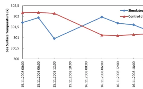
Figure 3. Comparison of best model performance (simulation 6) with control data, for 6-hourly SST prediction during typhoon Noul.

2.3 Verification process

After selecting the best simulation for each parameter in the case of typhoon Noul, the solutions were evaluated by run-ning the model for seven other typhoons, Peipah in 2007, Tropical Depression 01W in 2008, Kujira in 2009, Chan-Hom in 2009, Nangka in 2009, Songda in 2011, and Washi in 2011. The aim was to confirm the scheme selection pro-cesses for each parameter. The typhoons were selected from all storm track data set by Knapp et al. (2010).

3 Results and discussions

The data used for validation of the variables was derived from the CFSR data set and is available on the related website (Saha et al., 2010). The results from the nested domain were used for purposes of analysis and comparison.

3.1 Sea-surface temperature

Statistical evaluation of SST is presented in Table 2. The best result of the SST simulation is shown in bold. It can be noted that simulation 6 works satisfactorily for SST, because all criteria are met, with the exception of the CC value, which was lower than expected.

(5)

Table 3. Statistical evaluation of different simulations for LHF.

RMSE 95.75 115.2 112.6 140.8 143.9 168.9

CC 0.69 0.49 0.61 0.21 0.51 0.53

MBE −2.96 13.39 −22.67 31.56 −49.65 −16.28

tstatistic 0.15 0.59 1.04 1.17 1.87 0.49

26 1

2

LHF prediction during typhoon Noul

3 4 0 100 200 300 400 500 600 700 12 .11.20 08 06: 00 12 .11.20 08 12: 00 12 .11.20 08 18: 00 13 .11.20 08 00: 00 13 .11.20 08 06: 00 13 .11.20 08 12: 00 13 .11.20 08 18: 00 14 .11.20 08 00: 00 14 .11.20 08 06: 00 14 .11.20 08 12: 00 14 .11 .20 08 18: 00 15 .11.20 08 00: 00 15 .11.20 08 06: 00 15 .11.20 08 12: 00 15 .11.20 08 18: 00 16 .11.20 08 00: 00 16 .11.20 08 06: 00 16 .11 .20 08 12: 00 16 .11.20 08 18: 00 17 .11.20 08 00: 00 17 .11.20 08 06: 00 17 .11.20 08 12: 00 17 .11.20 08 18: 00 18 .11.20 08 00: 00 18 .11.20 08 06: 00 18 .11.20 08 12: 00 18 .11.20 08 18: 00 19 .11.20 08 00: 00 19 .11.20 08 06: 00 Late n t h e at fl u x (W/m 2) Time Simulated Control data

Figure 4. Comparison of best model performance (simulation 1) with control data, for 6-hourly LHF prediction during typhoon Noul.

typhoon is stronger, and under-prediction when the typhoon is weaker.

The spotlight of simulation 6 was the amount of tem-perature and moisture in the different atmospheric layers that were connected (Liu et al., 1997). Thus, this combina-tion could predict SST satisfactorily, comparing to the other groups in this paper.

3.2 Latent heat flux

The oceanic LHF is heat energy released or absorbed by the ocean during a phase transition without a change in temper-ature, such as water-surface evaporation (Clark, 2004).

As shown in Table 3, simulation 1 performs best for LHF prediction, with the minimum RMSE, MBE, and t values, and the maximum amount of CC.

Figure 4 shows a comparison of simulated and control data for LHF in the case of the best performing simulation. Although there are some over-prediction and some under-prediction points, it can be seen that most simulated values are very close to the control values.

In this study, the simulation number 1 has focused on the different water phases in clouds. Phase changing in the dif-ferent layers can affect the amount of LHF (Zhu and Zhang, 2006).

Table 4. Statistical evaluation of different simulations for SHF.

RMSE 58.37 30.89 60.71 64.48 23.69 54.62

CC 0.60 0.88 0.72 −0.02 0.93 0.524

MBE −12.85 −9.25 −22.38 −7.77 0.48 −14.38

tstatistic 1.15 1.6 2.02 1.77 0.03 1.39

27

1

2

SHF prediction during typhoon Noul

3 4 -60 -35 -10 15 40 65 12 .11.20 08 06: 00 12 .11.20 08 12: 00 12 .11.20 08 18: 00 13 .11.20 08 00: 00 13 .11.20 08 06: 00 13 .11.20 08 12: 00 13 .11.20 08 18: 00 14 .11 .20 08 00: 00 14 .11.20 08 06: 00 14 .11.20 08 12: 00 14 .11.20 08 18: 00 15 .11.20 08 00: 00 15 .11.20 08 06: 00 15 .11.20 08 12: 00 15 .11.20 08 18: 00 16 .11.20 08 00: 00 16 .11.20 08 06: 00 16 .11.20 08 12: 00 16 .11 .20 08 18: 00 17 .11.20 08 00: 00 17 .11.20 08 06: 00 17 .11.20 08 12: 00 17 .11.20 08 18: 00 18 .11.20 08 00: 00 18 .11.20 08 06: 00 18 .11.20 08 12: 00 18 .11.20 08 18: 00 19 .11.20 08 00: 00 Se n si b le h e at fl u x (W/m 2) Time Simulated Control data

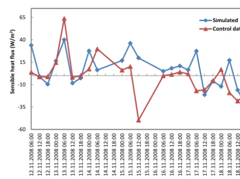
Figure 5. Comparison of best model performance (simulation 5) with control data, for 6-hourly SHF prediction during typhoon Noul.

3.3 Sensible heat flux

SHF is heat energy transferred by conduction and convection at the atmosphere–ocean interface that creates a change in the system temperature (Clark, 2004).

As shown in Table 4, of the six simulations, number 5 can strongly predict the SHF values with the highest value of CC (0.93).

The result of simulation 5, indicating its superior perfor-mance over others, is shown in Fig. 5. Almost all increasing and decreasing SHF values are predicted as well.

3.4 Precipitation rate

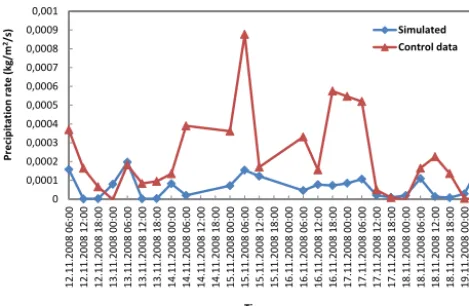
In the case of the precipitation rate, simulation 5 was the best-performing simulation, with consistently lowest RMSE, MBE, andt values, and the highest CC values, as shown in Table 5.

The simulated data from simulation 5 are compared with control data in Fig. 6. The results indicate that forecasts of precipitation rates before and after the typhoon are close to those of the control data. During the period of 14 to 17 November, the simulated data values for the typhoon were lower than the control data.

(6)

28

1

Fig. 6Comparison of best model performance (simulation 5) with control data, for six-hourly

2

precipitation rate prediction during typhoon Noul

3 4 0 0,0001 0,0002 0,0003 0,0004 0,0005 0,0006 0,0007 0,0008 0,0009 12 .11.20 08 06: 00 12 .11.20 08 12: 00 12 .11.20 08 18: 00 13 .11.20 08 00: 00 13 .11.20 08 06: 00 13 .11.20 08 12: 00 13 .11.20 08 18: 00 14 .11.20 08 00: 00 14 .11.20 08 06: 00 14 .11.20 08 12: 00 14 .11.20 08 18: 00 15 .11.20 08 00: 00 15 .11.20 08 06: 00 15 .11.20 08 12: 00 15 .11.20 08 18: 00 16 .11.20 08 00: 00 16 .11.20 08 06: 00 16 .11.20 08 12: 00 16 .11.20 08 18: 00 17 .11.20 08 00: 00 17 .11.20 08 06: 00 17 .11 .20 08 12: 00 17 .11.20 08 18: 00 18 .11.20 08 00: 00 18 .11.20 08 06: 00 18 .11.20 08 12: 00 18 .11.20 08 18: 00 19 .11.20 08 00: 00 19 .11 .20 08 06: 00 Pr e ci p itat io n r ate (k g/ m 2/s) Time Simulated Control data

Figure 6. Comparison of best model performance (simulation 5) with control data, for 6-hourly precipitation rate prediction during typhoon Noul.

combination has considered convection, mass flux, and cloud effects. Furthermore, Li (2013) demonstrated that the KF cu-mulus parameterization could create the most severe vertical convection.

3.5 Wind speed

Wind-speed estimations during the typhoon were statistically evaluated, as shown in Table 6. In spite of simulation 4 hav-ing low CC values, RMSE, and MBE, values are lower in comparison with those obtained in other simulations, and this simulation therefore shows the best performance for wind-speed prediction. Moreover, simulation number 4 focuses on mixed phase and multiband efficiency, along with the tem-perature, and the turbulent kinetic energy played a signifi-cant role in forecasting wind speed. According to Draxl et al. (2010), turbulent kinetic energy can perform well in pre-dicting wind speed.

A general tendency for the model to over-predict wind speed was noted in all simulations, and was also observed in many earlier studies (Hanna et al., 2010; Ruiz et al., 2010). Figure 7 shows the comparison between simulated wind speed and related control data. As noted in earlier stud-ies, wind speed is significantly affected by local fluctuations, especially in highly unstable conditions. Thus, wind sensitiv-ities tend to have more variation (Hu et al., 2010).

3.6 Verification process

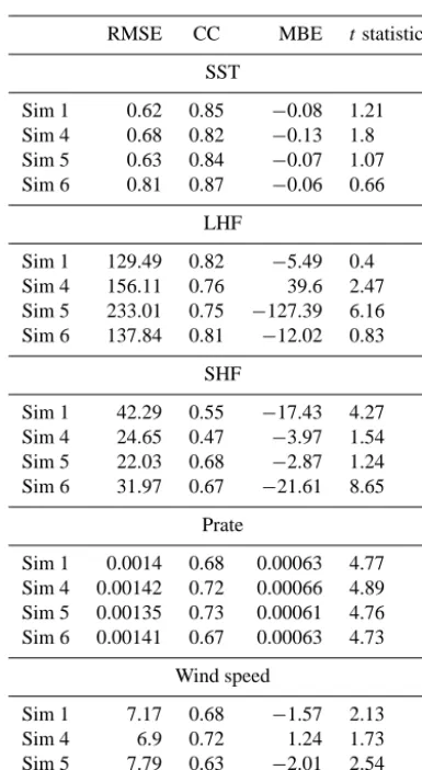
Herein, to find whether the best combinations are applicable or not, they were examined for seven other typhoons (named in Sect. 2.3). The calculated values of RMSE, CC, MBE, and t for these typhoons confirms that the suggested combina-tions show the same results, which are given in Table 7.

29

1

Fig. 7Comparison of best model performance (simulation 4) with control data, for six-hourly 2

wind speed prediction during typhoon Noul 3 4 0 2 4 6 8 12 .11.20 08 06: 00 12 .11.20 08 12: 00 12 .11.20 08 18: 00 13 .11.20 08 00: 00 13 .11.20 08 06: 00 13 .11.20 08 12: 00 13 .11.20 08 18: 00 14 .11.20 08 00: 00 14 .11.20 08 06: 00 14 .11.20 08 12: 00 14 .11.20 08 18: 00 15 .11.20 08 00: 00 15 .11.20 08 06: 00 15 .11.20 08 12: 00 15 .11.20 08 18: 00 16 .11 .20 08 00: 00 16 .11.20 08 06: 00 16 .11.20 08 12: 00 16 .11.20 08 18: 00 17 .11.20 08 00: 00 17 .11.20 08 06: 00 17 .11.20 08 12: 00 17 .11.20 08 18: 00 18 .11.20 08 00: 00 18 .11.20 08 06: 00 18 .11.20 08 12: 00 18 .11.20 08 18: 00 19 .11.20 08 00: 00 19 .11.20 08 06: 00 Wi n d sp e e d ( m /s) Time Simulated Control data

Figure 7. Comparison of best model performance (simulation 4) with control data, for 6-hourly wind-speed prediction during ty-phoon Noul.

3.7 Comparison with other studies for the wind speed prediction issue

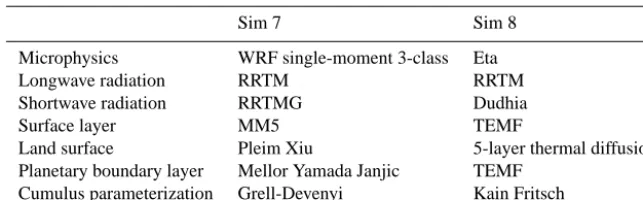
In this part, two sets of simulations were defined according to the previous studies by Chandrasekar and Balaji (2012), and Angevine (2010), which were considered as the best physics options for wind prediction. The simulations are indicated by abbreviations of Sim 7, and Sim 8, respectively. The details of their represented physics options are indicated in Table 8. These two suggested simulations for best wind predicting were conducted for typhoon Washi in 2011. The best wind-speed prediction by WRF model (simulation 4), CFSR data set, and these new simulations are compared (Fig. 8).

According to Fig. 8, the best physics options that were suggested for predicting typhoon intensity during this study (WRF) and also Sim 7 are nearly in the range of CFSR data set, and Sim 8 predicted stronger winds at some points.

4 Conclusions

From the results obtained, it is evident that there is no sin-gle combination of physics options that performs best for all desired parameters. However, the present study suggests suitable options for different variables, when considering ty-phoon existence in the South China Sea. According to differ-ent schemes defined in this paper, SST, LHF, SHF, precipita-tion rate, and wind speed are best estimated by simulaprecipita-tions 6, 1, 5, 5, and 4, respectively. Therefore, the model configura-tion should be chosen from the viewpoint of the objective of the study being undertaken. The main conclusions of this study are as follows:

(7)

Table 5. Statistical evaluation of different simulations for precipitation rate.

RMSE 0.00027 0.00028 0.00026 0.00028 0.00025 0.00026

CC 0.329 0.105 0.264 0.369 0.405 0.301

MBE 0.00017 0.00017 0.00016 0.00018 0.00015 0.00016

tstatistic 4.085 4.062 3.841 4.414 3.699 3.943

Table 6. Statistical evaluation of different simulations for wind speed.

RMSE 4.28 3.87 4.10 3.11 4.39 3.15

CC 0.42 0.37 0.49 0.41 0.57 0.70

MBE −2.69 −2.01 −2.93 −1.64 −3.09 −2.18

tstatistic 4.13 3.10 5.20 3.17 5.07 4.91

Table 7. The values of statistic parameters for confirming the best combinations suggested for the selected parameters.

RMSE CC MBE tstatistic

SST

Sim 1 0.62 0.85 −0.08 1.21

Sim 4 0.68 0.82 −0.13 1.8

Sim 5 0.63 0.84 −0.07 1.07

Sim 6 0.81 0.87 −0.06 0.66

LHF

Sim 1 129.49 0.82 −5.49 0.4

Sim 4 156.11 0.76 39.6 2.47

Sim 5 233.01 0.75 −127.39 6.16

Sim 6 137.84 0.81 −12.02 0.83

SHF

Sim 1 42.29 0.55 −17.43 4.27

Sim 4 24.65 0.47 −3.97 1.54

Sim 5 22.03 0.68 −2.87 1.24

Sim 6 31.97 0.67 −21.61 8.65

Prate

Sim 1 0.0014 0.68 0.00063 4.77

Sim 4 0.00142 0.72 0.00066 4.89

Sim 5 0.00135 0.73 0.00061 4.76

Sim 6 0.00141 0.67 0.00063 4.73

Wind speed

Sim 1 7.17 0.68 −1.57 2.13

Sim 4 6.9 0.72 1.24 1.73

Sim 5 7.79 0.63 −2.01 2.54

Sim 6 7.38 0.67 −1.95 2.6 30

1

Fig. 8 Comparison wind speed prediction for typhoon Washi by different simulations and data 2

sets 3

4

0,00 5,00 10,00 15,00 20,00 25,00 30,00

15

.12

.20

11

18:

00

16

.12.20

11 00:

00

16

.12.20

11 06:

00

16

.12.20

11 12:

00

16

.12.20

11 18:

00

17

.12.20

11 00:

00

17

.12.20

11 06:

00

17

.12.20

11 12:

00

17

.12.20

11 18:

00

18

.12.20

11 00:

00

18

.12.20

11 06:

00

18

.12.20

11 12:

00

18

.12.20

11 18:

00

Wi

n

d

sp

e

d

(

m

/s)

Time

WRF

CFSR

Sim7

Sim8

Figure 8. Comparison of wind-speed prediction for typhoon Washi through different simulations and data sets.

– The recommended combinations of physics options for the mentioned parameters were confirmed with seven other typhoons.

– Comparing the presented best simulations with the CFSR database showed that the suggested groups can be applicable in predicting issues except for precipita-tion rate.

– Overall, the performance of the WRF model is accept-able and satisfactory for prediction of important param-eters related to typhoon intensity over the South China Sea region.

(8)

Sim 7 Sim 8

Microphysics WRF single-moment 3-class Eta

Longwave radiation RRTM RRTM

Shortwave radiation RRTMG Dudhia

Surface layer MM5 TEMF

Land surface Pleim Xiu 5-layer thermal diffusion

Planetary boundary layer Mellor Yamada Janjic TEMF

Cumulus parameterization Grell-Devenyi Kain Fritsch

Acknowledgements. This study was supported by a fellowship

of Centre for Marine and Coastal Studies (CEMACS), Universiti Sains Malaysia.

Edited by: P. Nastos

Reviewed by: two anonymous referees

References

Angevine, W. M.: The Total Energy-Mass Flux PBL scheme in WRF: Experience in real-time forecasts for California, 19th Symposium on Boundary Layers and Turbulence, Colorado, 2010.

Ardie, W. A., Sow, K. S., Tangang, F. T., Hussin, A. G., Mahmud, M., and Juneng, L.: The performance of different cumulus pa-rameterization schemes in simulating the 2006/2007 southern peninsular Malaysia heavy rainfall episodes, J. Earth Syst. Sci., 121, 317–327, 2012.

Betts, A. and Miller, M.: A new convective adjustment scheme, Part II: Single column tests using GATE wave, BOMEX, ATEX and arctic air-mass data sets, Q. J. Roy. Meteorol. Soc., 112, 693– 709, 1986.

Chandrasekar, R. and Balaji, C.: Sensitivity of tropical cyclone Jal simulations to physics parameterizations, J. Earth Syst. Sci., 121, 923–946, 2012.

Clark, J. O. E.: The essential dictionary of science, Barnes & Noble Books, New York, 2004.

Draxl, C., Hahmann, A. N., Pena Diaz, A., Nissen, J. N., and Giebel, G.: Validation of boundary-layer winds from WRF mesoscale forecasts with applications to wind energy forecast-ing, 19th Symposium on Boundary Layers and Turbulence, Col-orado, 2010.

Dudhia, J.: Numerical study of convection observed during the winter monsoon experiment using a mesoscale two-dimensional model, J. Atmos. Sci., 46, 3077–3107, 1989.

Gilliam, R. C. and Pleim, J. E.: Performance assessment of new land surface and planetary boundary layer physics in the WRF-ARW, J. Appl. Meteorol. Clim., 49, 760–774, 2010.

Han, J. and Pan, H. L.: Revision of convection and vertical diffusion schemes in the NCEP global forecast system, Weather Forcast., 26, 520–533, 2011.

Hanna, S. R., Reen, B., Hendrick, E., Santos, L., Stauffer, D., Deng, A., McQueen, J., Tsidulko, M., Janjic, Z., and Jovic, D.: Com-parison of observed, MM5 and WRF-NMM model-simulated, and HPAC-assumed boundary-layer meteorological variables for 3 days during the IHOP field experiment, Boundar-Lay. Meteo-rol., 134, 285–306, 2010.

Ho, C. R., Zheng, Q., Soong, Y. S., Kuo, N. J., and Hu, J. H.: Sea-sonal variability of sea surface height in the South China Sea ob-served with TOPEX/Poseidon altimeter data, J. Geophys. Res., 105, 981–990, 2000.

Hong, S. Y., Dudhia, J., and Chen, S. H.: A revised approach to ice microphysical processes for the bulk parameterization of clouds and precipitation, Mon. Weather Rev., 132, 103–120, 2004. Hong, S. Y., Noh, Y., and Dudhia, J.: A new vertical diffusion

pack-age with an explicit treatment of entrainment processes, Mon. Weather Rev., 134, 2318–2341, 2006.

Hu, X. M., Nielsen-Gammon, J. W., and Zhang, F.: Evaluation of three planetary boundary layer schemes in the WRF model, J. Appl. Meteorol. Clim., 49, 1831–1844, 2010.

Jacovides, C. and Kontoyiannis, H.: Statistical procedures for the evaluation of evapotranspiration computing models, Agr. Water. Manage., 27, 365–371, 1995.

Janjic, Z. I.: The step-mountain eta coordinate model: Further de-velopments of the convection, viscous sublayer, and turbulence closure schemes, Mon. Weather Rev., 122, 927–945, 1994. Jin, J., Miller, N. L., and Schlegel, N.: Sensitivity study of four land

surface schemes in the WRF model, Adv. Meteorol., 2010, 1–11, doi:10.1155/2010/167436, 2010.

JTWC: Best Track Data Set, available at: http://www.usno.navy. mil/JTWC/2008 (last access: 1 September 2012), 2008. Kain, J. S.: The Kain-Fritsch convective parameterization: an

up-date, J. Appl. Meteorol., 43, 170–181, 2004.

Knapp, K. R., Kruk, M. C., Levinson, D. H., Diamond, H. J., and Neumann, C. J.: The international best track archive for climate stewardship (IBTrACS) unifying tropical cyclone data, B. Am. Meterol. Soc., 91, 363–376, 2010.

Kwun, J. H., Kim, Y.-K., Seo, J. W., Jeong, J. H., and You, S. H.: Sensitivity of MM5 and WRF mesoscale model predictions of surface winds in a typhoon to planetary boundary layer parame-terizations, Nat. Hazards, 51, 63–77, 2009.

(9)

Lin, Y. and Colle, B. A.: A new bulk microphysical scheme that includes riming intensity and temperature-dependent ice charac-teristics, Mon. Weather Rev., 139, 1013–1035, 2011.

Lin, Y. L., Farley, R. D., and Orville, H. D.: Bulk parameterization of the snow field in a cloud model, J. Clim. Appl. Meteorol., 22, 1065–1092, 1983.

Liu, Y., Zhang, D. L., and Yau, M.: A multiscale numerical study of Hurricane Andrew (1992), Part I: Explicit simulation and verifi-cation, Mon. Weather Rev., 125, 3073–3093, 1997.

Mandal, M., Mohanty, U., and Raman, S.: A study on the impact of parameterization of physical processes on prediction of tropi-cal cyclones over the Bay of Bengal with NCAR/PSU mesostropi-cale model, Nat. Hazards, 31, 391–414, 2004.

Menéndez, M., Tomás, A., Camus, P., Garcia-Diez, M., Fita, L., Fernandez, J., Méndez, F., and Losada, I.: A methodology to evaluate regional-scale offshore wind energy resources, Oceans, IEEE, Spain, 1–8, 2011.

Michalakes, J., Dudhia, J., Gill, D., Henderson, T., Klemp, J., Ska-marock, W., and Wang, W.: The weather research and forecast model: software architecture and performance, Proceedings of the 11th ECMWF Workshop on the Use of High Performance Computing In Meteorology, 156–168, 2004.

Mlawer, E. J., Taubman, S. J., Brown, P. D., Iacono, M. J., and Clough, S. A.: Radiative transfer for inhomogeneous atmo-spheres: RRTM, a validated correlated-k model for the longwave, J. Geophys. Res., 102, 16663–16682, 1997.

Mohan, M. and Bhati, S.: Analysis of WRF Model Performance over Subtropical Region of Delhi, India, Adv. Meteorol., 2011, 621235.1–621235.13, 2011.

NOAA: Best track data set [Online], available at: http://www.csc. noaa.gov/hurricanes/2008 (last access: 1 September 2012), 2008. Pleim, J. E.: A combined local and nonlocal closure model for the atmospheric boundary layer, Part I: Model description and test-ing, J. Appl. Meteorol. Clim., 46, 1383–1395, 2007.

Rahmstorf, S.: A fast and complete convection scheme for ocean models, Ocean Model., 101, 9–11, 1993.

Rogers, E., Black, T., Ferrier, B., Lin, Y., Parrish, D., and Dimego, G.: Changes to the NCEP Meso Eta Analysis and Fore-cast System: Increase in resolution, new cloud microphysics, modified precipitation assimilation, modified 3DVAR analysis, NWS Tech. Procedures Bull. 488, http://www.emc.ncep.noaa. gov/mmb/mmbpll/eta12tpb/, last access: August 2014, 1–15, 2001.

Ruiz, J. J., Saulo, C., and Nogués-Paegle, J.: WRF model sensitiv-ity to choice of parameterization over South America: validation against surface variables, Mon. Weather. Rev., 138, 3342–3355, 2010.

Saha, S., Moorthi, S., Pan, H. L., Wu, X., Wang, J., Nadiga, S., Tripp, P., Kistler, R., Woollen, J., Behringer, D., Liu, H., Stokes, D., Grumbine, R., Gayno, G., Wang, J., Hou, Y. T., Chuang, H. Y., Juang, H. M. H., Sela, J., Iredell, M., Treadon, R., Kleist, D., Van Delst, P., Keyser, D., Derber, J., Ek, M., Meng, J., Wei, H., Yang, R., Lord, S., Van Den Dool, H., Kumar, A., Wang, W., Long, C., Chelliah, M., Xue, Y., Huang, B., Schemm, J.-K., Ebisuzaki, W., Lin, R., Xie, P., Chen, M., Zhou, S., Higgins, W., Zou, C. Z., Liu, Q., Chen, Y., Han, Y., Cucurull, L., Reynolds, R. W., Rutledge, G., and Goldberg, M.: NCEP Climate Forecast System Reanalysis (CFSR) 6-hourly Products, January 1979 to December 2010, Research Data Archive at the National Center for Atmospheric Research, Computational and Information Sys-tems Laboratory, Boulder, CO, 2010.

Skamarock, W. C., Klemp, J. B., Dudhia, J., Gill, D. O., Barker, D. M., Wang, W., and Powers, J. G.: A description of the advanced

research WRF version 2, http://oai.dtic.mil/oai/oai?verb=

getRecord&metadataPrefix=html&identifier=ADA487419, NCAR, Boulder, Colorado, 101 pp., 2005.

Tao, W. K. and Simpson, J.: The Goddard cumulus ensemble model, Part I: Model description, Terr. Atmos. Ocean. Sci., 4, 35–72, 1993.

Tao, W. K., Anderson, D., Atlas, R., Chern, J., Houser, P., Hou, A., Lang, S., Lau, W., Peters-Lidard, C., and Kakar, R.: A Goddard Multi-Scale Modeling System with Unified Physics, WCRP/GEWEX Newslett., 18, 6–8, 2008.

Thompson, G., Field, P. R., Rasmussen, R. M., and Hall, W. D.: Explicit forecasts of winter precipitation using an improved bulk microphysics scheme, Part II: Implementation of a new snow pa-rameterization, Mon. Weather Rev., 136, 5095–5115, 2008. Tiedtke, M.: A comprehensive mass flux scheme for cumulus

pa-rameterization in large-scale models, Mon. Weather Rev., 117, 1779–1800, 1989.

Wang, W., Bruyere, C., Duda, M., Dudhia, J., Gill, D., Lin, H., Michalakes, J., Rizvi, S., Zhang, X., and Beezley, J.: ARW mod-eling system user’s guide. Mesoscale & Miscroscale Meteorol-ogy Division (version 3), National Center for Atmospheric Re-search, Boulder, USA, 2010.

Yang, L., Li, W.-W., Wang, D., and Li, Y.: Analysis of Tropical Cy-clones in the South China Sea and Bay of Bengal during Mon-soon Season, in: Recent Hurricane Research – Climate, Dynam-ics, and Societal Impacts, edited by: Lupo, P. A., InTech, Croatia and China, 616 pp., 2011.

Zhang, C., Wang, Y., and Hamilton, K.: Improved Representation of Boundary Layer Clouds over the Southeast Pacific in ARW-WRF Using a Modified Tiedtke Cumulus Parameterization Scheme, Mon. Weather Rev., 139, 3489–3513, 2011.