THE STUDY OF LINEARIZED
DISTURBANCES IN A STRATIFIED
BOUNDARY LAYER
Vijayalakshmi A.R.
Department of Mathematics, Maharani’s Science College for women, Palace road, Bangalore – 560 001, INDIA
E-mail: [email protected]
Abstract: The evolution of linearized disturbances in a stratified shear flow is studied by making use of the initial value problem approach. The resulting equation in time posed by using Fourier transform is solved for the Fourier amplitudes for the case of boundary layer flow. The initial distributions that are considered are a point source of the field of transverse velocity and density. For small values of Brunt
V
a
is
a
l
a
frequency the perturbation solutions are obtained.Key words: Stratified shear flow, initial value problem, fourier transform, Brunt
V
a
is
a
l
a
frequency.1. Introduction
The stability of stratified shear flow has been investigated by many researchers. Eliassen, Hoiland and Riis (1953) considered flow between two parallel walls. By using initial-value problem approach they showed that a disturbance originating from arbitrary initial conditions would behave
asymptotically like
γ
1
2
1
t
,
2
1
J
4
-1
γ
for3
J
0
1
4
4
but would be exponentially unstable for Richardson number,J
0
3
4
, for the semi-infinite case. Case (1960) gave a rather complete stability analysis for the problem of a semi – infinite exponential atmosphere. A sufficient condition for stability in a parallel stratified, inviscid flow that the local Richardson number0
J
should everywhereexceed
4
1
was established by [Miles (1961]). [Kuo (1963)] studied small perturbations of plane Couetteflow in stably and unstably stratified fluids and found that the system to be more unstable when it is bounded both above and below than when its depth is infinite.[Chimonas (1979)] studied the stability of stratified shear flow and concluded that the flow will be unstable if the local Richardson number falls
below
4
1
anywhere in the flow. The problem of stability of plane Couette flow is plagued byalgebraically decaying disturbances that are less easily handled than exponentially decaying (or growing) modes. [Brown and Stewartson (1980)] have resolved the controversy surrounding the decay rate in favour of original results of [Eliassen et al (1953)].
In this paper, we have extended the work of [Criminale and Drazin (1990)], for the case of stratified boundary layer. Taking a multilayered basic flow with piecewise linear velocity profile, complete general solutions to the linearized equations of motion are obtained as functions of all space variables and time, when posed as initial-value problems. The distributions are resolved into two components, rotational and irrotational. The solution for the hypothetical initial-value problem for which the basic flow is unbounded but coincides with the actual flow in the layer is the rotational solution. The irrotational solution in each layer is specified uniquely by satisfying the interfacial conditions and boundary conditions at a wall or at infinity. [Vijayalakshmi and Balagondar, (2014)] studied the evolution of linearized perturbations in a magnetohydrodynamic boundary layer.
2. MATHEMATICAL FORMULATION
We consider an inviscid, incompressible fluid of density moving with velocity
q
under the influence of gravityg
directed in the negative y-direction. We assume that the fluid is inviscid, incompressible, stratified and is Boussinesq for which motion is governed by the equations0
q
.
q
.
q
-
p
ρ
g
t
q
ρ
, (2.2)
q
.
ρ
0
t
ρ
, (2.3)
where p is the pressure.
In the basic unperturbed equilibrium state,
U
y
σ
y,
0,
0
0
q
,p
p
0
y
,ρ
ρ
0
y
(2.4)where , the intensity shear is constant.
For linear stability analysis, we superimpose a small perturbation upon the mean flow i,e.,
q
0
q
q
,p
p
0
y
p
,ρ
ρ
0
y
ρ
(2.5)where
q
,p
andρ
are the perturbed quantities of velocity, pressure and density respectively.To study the evolution of linearized perturbations in a stratified shear flow, we linearize Eq.(2.1)–(2.3) using Eq.(2.5). The linearized differential equations of motion (neglecting the primes), by (i) employing moving co-ordinates transformation,
z
ζ
y,
η
y t,
σ
-x
ξ
t,
T
, (2.6)(ii) employing three - dimensional Fourier transformation of the form
α
;
β
;
γ
;
T
u
ξ
;
η
;
ζ
;
T
e
i
α
ξ
βη
γ
ζ
d
ξ
d
η
d
ζ
uˆ
,with similar expressions for
vˆ
,wˆ
,pˆ
andρ
ˆ
,(2.7)
(iii)expressing the velocity components in the
α
andφ
directions as (2.23)α
wˆ
α
uˆ
γ
w
,
α
wˆ
γ
uˆ
α
u
(2.8)and eliminating
pˆ
, the set of equations (2.1)–(2.3) is reduced to a differential equation of the form
K
2
vˆ
N
2
α
2
vˆ
0
2
dT
2
d
, (2.9)
where
K
2
α
2
β
σα
T
2
andα
2
α
2
γ
2
.dy
0
ρ
d
0
ρ
g
2
N
,ρ
0
is the equilibrium density, N is the BruntV
a
is
a
l
a
frequency.Two sets of solutions exist for Eq.(2.9), when
K
2
0
, the disturbance is rotational and for0
2
K
, the disturbance is irrotational. The vanishing of the productK
2
vˆ
corresponds to Laplaceequation
2
vˆ
0
in real space. We denotevˆ
asvˆ
R
whenK
2
0
which is called the rotational solution andvˆ
asI
vˆ
whenK
2
0
and is called the irrotatioal solution. Thereforevˆ
can be resolved into two components and thusvˆ
vˆ
R
vˆ
I
.
α
,
β
,
γ
,
T
vˆ
0
α
,
β
,
γ
,
T
N
2
vˆ
1
α
,
β
,
γ
,
T
N
2
2
vˆ
2
α
,
β
,
γ
,
T
...
R
vˆ
(2.10)where
R
vˆ
is the rotational component ofvˆ
.At the zeroth,first and second order solutions are found .
ˆ
ˆ
ˆ
ˆ
T
Ω
α
,
β
,
γ
Ω α
,
β
,
γ
2 2
βΩ
Ω
β σα
T
0
1
0
1
ˆv
α
N
R
α
2
β σα
T
2
σ α α
2 2
σαα
α
12
2
2
2
α
β σα
T
α
β σα
T
β σα
T
α
1
β σα
T
tan
log log
2
2
α
2
σ
α
α
2
σ
α
α
ˆ
3
Ω
2
β σα
T
1
β σα
T
0
1
2
α
2 -tan
N
2 2 2
2
2
α
α
σ α α
α
β σα
T
σα
ˆ
ˆ
2
2
Ω
0
Ω
1
1
β σα
T
1
β σα
T
α
β σα
T
β σα
T
tan
log
2
2 2
σαα
2 2
α
α
2
α
σ α α
2
σ α
α
2
2
2
4
2
2
α
β σα
T
α
β σα
T
β σα
T
β σα
T
1
1
1
1
tan
log log
2
2
2
α
2
α
α
12
σαα
α σαα
α
σα
T
β
1
tan
α
σα
T
β
2
2
2
α
2
σα
T
β
2
α
log
α
σα
T
β
α
4
α
4
8
σ
0
Ω
ˆ
3
α
σα
T
β
3
1
2
α
2
σα
T
β
2
α
log
α
σα
T
β
1
tan
α
σα
T
β
2
2
α
2
σα
T
β
2
α
log
α
σα
T
β
1
tan
2
α
2
σ
2
α
σα
T
β
1
tan
α
σα
T
β
2
2
α
2
σα
T
β
2
α
log
α
σα
T
β
α
3
α
4
2
σ
0
Ω
ˆ
β
σα
T
2
2
α
1
α
σα
T
β
1
tan
sin
α
σα
T
β
1
tan
cos
. (2.11)The solution for
K
2
0
which corresponds to irrotational motion is obtained by considering the two– dimensional Fourier transform of the perturbation equations instead of the full three–dimensional decomposition. Using moving co-ordinate transformation given by Eq. (2.6),K
2
vˆ
0
corresponds to
α
2
σ
2
α
2
T
2
v
I
0
η
I
v
α
T
2i
σ
2
η
I
v
2
where
ξ
,
η
,
ς
,
T
e
i
αξ
γζ
d
ξ
d
ζ
I
v
T
γ
;
η
,
α
,
I
v
I
v
, (2.13)is the irrotational part of
vˆ
. The solution of Eq. (2.14) is found to be
T
e
α
η
i
σ
α
T
η
B
T
e
α
η
i
σ
α
T
η
A
I
v
, (2.14)
where A(T) and B(T) are constants of integration .
In order to combine
vˆ
R
andv
I
to obtain the complete the solution and satisfy the matching conditionvˆ
R
must be inverted once to obtainv
R
α
,
η
,
γ
;
T
i,e.,
vˆ
R
α
,
β
,
γ
;
T
e
-
i
β
η
d
β
2
π
1
T
γ
;
η
,
α
,
R
v
. (2.15)
With initial velocity and initial density as unit pulse, the initial conditions are expressed as
x,
y,
z,0
V
0
δ
x
-
x
0
δ
y
-
y
0
δ
z
-
z
0
v
. (2.16)
x,
y,
z,0
~
ρ
0
δ
x
-
x
0
δ
y
-
y
0
δ
z
-
z
0
ρ
. (2.17)In terms of moving co-ordinates and three-dimensional Fourier transform, Eq. (2.16) and Eq. (2.17) becomes
Ω
0
α
,
β
,
γ
V
0
e
i
α
x
0
β
y
0
γ
z
0
γ
β
,
α
,
0
v
. (2.18)
Ω
1
α
,
β
,
γ
~
ρ
0
e
i
α
x
0
β
y
0
γ
z
0
γ
β
,
α
,
0
ρ
~
. (2.19)R
v
is found to be
α
σα
1
1
α
σα
0
ρ
~
α
2
α
2
σ
0
V
2
α
2
12
σ
2
α
4
N
0
ρ
~
0
TV
η
α
e
η
σα
T
0
γ
z
0
α
x
i
e
R
v
4 3
4 4
2
α η
V
ρ
2i N
α
V
i N
α
V
e
0
0
2
4 4
0
0
N
2
α
N
-2
2 2
σαα
2 2
5 5
ηα
σ α α
σ α α
2
σ α
d
η
η
-
η
η
d
η
d
η
η
α
η
-η
α
η
-η
η
α
e
5
α
5
8
σ
4
N
2
α
0
2iV
α
4
α
4
8
σ
4
N
0
V
d
η
η
-η
η
α
η
η
α
e
2
α
2
σ
1
1
α
3
α
4
σ
4
N
0
iV
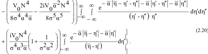
.
(2.20)
Here
η
η
-
y
0
. Now the complete solution will beI
v
R
v
v
. (2.21)R
v
andv
I
given by Eq.(2.21) and Eq.(2.14).3. STRATIFIED BOUNDARY LAYER FLOW
Fig. 1 Sketch of stratified boundary layer flow on a wall.
This problem consists of both plane Couette flow and the layered infinite flow i,e., wall layer (or shear layer) and the free stream. The model of the magnetohydrodynamic boundary layer is as shown in Fig. 1.
In the free stream, the moving co-ordinate system for a constant mean flow
U
0
is given by
T
t,
ξ
x
-
U
0
t,
η
y,
ζ
z
. (3.1) The Fourier transforms and inversions follow as it has been done before. Thus
A
s
T
e
α
η
s
I
v
, (3.2)
3
2
i
α
x
0
γ
z
0
e
αη
2 2
T V
0
0
T
v
R
e
TV
0
0
6
2
s
N
5 4
T V T
4 2 0 0
120 24
N
(3.3)
y
η
for
y
H
0
U
H
y
for
σ
y
y
U
The subscript s denotes the quantities in the free stream. In the wall layer,
v
R
andv
I
are given by Eq. (2.21) and Eq. (2.14).We have
v
= 0 at the solid boundaryη
= 0. Thus,
A B
- A
3
T
B
3
e
i
α
x
0
γ
z
0
σα
Ty
0
(3.4)We make use of kinematic condition and pressure matching conditions.
velocity
v
must be continuous at the interfaceη
= H, i,e.,
v
η
H
H
η
s
v
gives
α
H
i
α
x
0
γ
z
0
α
H - y
0
α
H
α
H
i
σ
α
T H y
0
A T e
s
TV
0
ρ
0
e
Ae
Be
e
A T + B e
i
α
x
0
γ
z
0
σα
T H - y
0
1
1
. (3.5)Pressure
Pˆ
must be continuous at the interfaceη
= H,i,e.,
H
η
layer
wall
p
H
η
stream
free
p
gives
αη
0
0
2 3
α
0
-
α
A T e
s
V
0
α
0
TV
0
ρ
0
- V
0
2
α
i
x
z
H y
e
N
H
y
e
01
2 α
T V α α
4α 0 ρ 0 1 α eiσα TH
0 2
H y H y
N T e
e
d
F
αH αH
α
H
α
H
i
σ
α
TH
-A e
Be
i
σ
α
1
α
H Ae
i
σ
α
1
α
H Be
e
. (3.6)From Eq.(3.5) and Eq,(3.6), we obtain
2
α
H
α
H
2
α
H
α
H
α
H
A
e
e
A e
e
e
3
3
1
1
3
1
B
2
2
α
H
2
α
1- 2
α
H e
2
α
H
1-2
α
H e
2
i
σ
α
y
0
σ
α
y
2
α
2
α
0
T
B
PT Q
P
+
A
1
1
i
σα
A
3
y T
0
i
A
1
y
0
α
H-i
σα
TH
e
2
2
α
H
2
α
H
1-2
α
H e
1-2
α
H e
2
i
σ
α
y
0
σ
α
y
2
2
0
B
H
H
H
H
2
α
H
2
α
H
i
σ
1- 2
α
H e
i
α
x
0
γ
z
0
σ
α
Ty
0
1- 2
α
H e
e
i
σ
+
α
y0
3
2
2
T
T
C e
Using B (0) = 0,
D
3
is found to be2
α
H
α
H
2
α
H
α
H
α
H
e
e
A e
e
e
3
1
3
1
C
3
2
2
α
H
2
α
1-2
α
H e
2
α
H
1-2
α
H e
2
i
σ
α
y
0
σ
α
y
2
α
2
α
0
B
Q
P
+
i
A
y
A
1
1
1
0
α
H
e
2
2
α
H
2
α
H
1-2
α
H e
1-2
α
H e
2
i
σ
α
y
0
σ
α
y
2
2
0
H
B
H
H
. (3.8)
Equation (3.4) yields,
i
α
x
0
γ
z
0
σ
α
Ty
0
α
0
A - A
3
T
B
3
e
e
y
B
. (3.9)The values of the coefficients are given in APPENDIX .
3. RESULTS AND DISCUSSIONS
In this problem, we have studied the evolution of linearized perturbations of a basic flow of an inviscid stratified boundary layer flow using piecewise linear velocity profiles. The initial disturbances used are unit pulse for velocity and density. In these broken line (piecewise linear) profiles, we have resolved the perturbations into rotational and irrotational components.
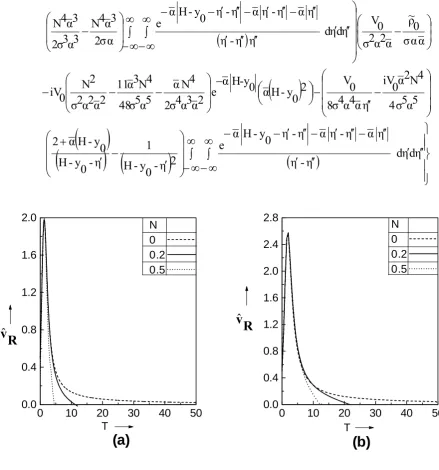
Figs. 2(a)–(b) are plots of
vˆ
R
versus T for different values of BruntV
a
is
a
l
a
frequency N (N = 0, 0.2, 0.5) andφ
(φ
0 , 45
0
0
). It is observed that as the value of N increasesvˆ
R
decays at a faster rate for large time. Hence we can conclude that stratification stabilizes the flow velocity but there is growth in the perturbation density.REFERENCES:
[1] Brown, S N, ; Stewartson K, (1980): On the algebraic decay of disturbances in a stratified linear shear flow. J. Fluid Mech, 100 ,pp 811- 816.
[2] Chimonas, G, (1979): Algebraic disturbances in stratified shear flows. J. Fluid Mech. 90,pp 1 - 9.
[3] Criminale, W O, and Drazin, P G, (1990): The Evolution of linearized perturbations of parallel flows. Stud. App. Math.83 (1990) pp 123 -147 .
[4] Eliassen A Holland E; Riis E, (1953): Two – dimensional perturbation of a flow with constant shear of a stratified fluid. Inst. Weather and Climate Res. Norwegian Acad. Sci. & Lett. Publ. No. 1.
[5] Kuo, H L,(1963): Perturbations of plane Couette flow in stratified fluid and origin of cloud streets, Phys. Fluids. 6, pp 195 - 211.
[6] Miles J W, (1961) :On the stability of heterogeneous shear flow. J. Fluid Mech. 10, pp 496 – 508.
[7] Vijayalakshmi, AR, ; Balagondar, PM, (2014): The Evolution of Linearized Perturbations in a Magnetohydrodynamic Boundary layer. Int J of Applied Mechanics and Engineering,19,2,pp 397-406.
APPENDIX
-
α
H - y
0
V e
,
1
0
A
3
1
,
3
1
0
0
A
A
B
B
H
H
2
α
4 2
0
α
0
N
α
V
0
ρ
0
1
e
V
0
ρ
0
B
1
e
ρ
0
2 2
2 2
1
2
2 2
σαα
σαα
σαα
12
σ α
σ α α
0
α
σ α α
H y
H y
H
y
2i N
4 3
α
V
i N
4 4
α
V
V
ρ
2
α
4 4
N
2
4 4
0
0
0
0
2
N
2
α
N
2 2
5 5
2 2
-N
α
σαα
σ
2
σ α
σ α α
σ α α
α
H-y
η α
η
α
H-y
0
η α
η
2
H - y
η
e
0
η
e
N
0
d
η
d
η
2
σ
η
H - y
0
η
2
3 4
4
α
V
ρ
N
11
α
N
α
N
0
0
0
V
0
H - y
0
e
2 2
2 2 2
5 5
4 3 2
σ α α
σαα
σ α α
48
σ α
2
σ α α
H y
i
α
H-y
η
-
η α
η
-
η α
η
4 3
4 3
0
N
α
N
α
e
d
η
d
η
+
3 3
2
σ
α
η
-
η
η
2
σ α
α
H - y
η
-
η
α
η
-
η
α
η
4
2 4
0
V N
0
2iV
0
α
N
e
d
η
d
η
5 5
4 4
8
σ α
H - y
η
-
η
η
-
η η
8
σ α α
0
α
H - y
η
α
η
4
0
iV N
0
1
e
1
d
η
4 3
2 2
H - y -
η
σ α α
σ α
0
e
-
α
H
-
y
0
0
y
H
α
2
σα
i
0
V
1
P
,
0
y
-H
-α
-e
0
y
H
α
2
σα
i
0
V
1
R
α
σα
1
1
α
σα
0
ρ
~
α
2
α
2
σ
0
V
2
α
2
12
σ
2
α
4
N
0
ρ
~
0
TV
0
y
-H
α
e
α
i
σ
0
V
α
-1
Q
5
α
5
2
σ
0
V
4
α
4
N
i
α
2
α
2
σ
0
V
3
α
4
N
2i
-4
N
4
α
2
2
N
α
σα
0
ρ
~
α
2
α
2
σ
0
V
2
α
0
y
-H
0
y
-H
α
2
e
σ
4
N
4
α
2
α
2
N
-α
σα
0
ρ
~
α
2
α
2
σ
0
V
η
α
η
0
y
-H
α
e
0
y
H
α
2
d
η
α
α
σ
0
ρ
~
α
2
α
2
σ
0
V
η
d
η
d
η
η
-η
η
α
η
-η
α
η
-η
0
y
-H
α
e
α
2
σ
3
α
4
N
3
α
3
2
σ
3
α
4
N
5
α
5
σ
4
4
N
2
α
0
iV
η
α
4
α
4
8
σ
0
V
2
0
y
-H
α
0
y
-H
α
e
2
α
3
α
4
2
σ
4
N
α
5
α
5
48
σ
4
N
3
α
11
2
α
2
α
2
σ
2
N
0
iV
η
d
η
d
η
-η
η
α
η
-η
α
η
-η
0
y
-H
α
e
2
η
-0
y
-H
1
η
-0
y
-H
0
y
-H
α
2
Fig. 2 Plots of
v
ˆ
R
versus T for (a)φ
0
o
and (b)φ
45
o
, for different values of N.0 10 20 30 40 50
0.0 0.4 0.8 1.2 1.6 2.0
N 0 0.2 0.5
(a)
T
R
v
ˆ
v
ˆ
R
0 10 20 30 40 50
0.0 0.4 0.8 1.2 1.6 2.0 2.4 2.8
N 0 0.2 0.5