Analysis of the Navigation Behavior of the
Users’ using Grey Relational Pattern
Analysis with Markov Chains
BINDU MADHURI .Ch* DR. ANAND CHANDULAL.J
Department of Computer Science & Engineering, GIT, Gitam University, INDIA
Abstract
Generally user page visits are sequential in nature. The large number of Web pages on many Web sites has raised navigational problems. Markov chains have been used to model user sequential navigational behavior on the World Wide Web (WWW).The enormous growth in the number of documents in the WWW increases the need for improved link navigation and path analysis models. Link prediction and path analysis are important problems with a wide range of applications ranging from personalization to websites. The complete size of the WWW coupled with the variation in users' navigation patterns makes this a very difficult sequence modeling problem. This paper generalizes the concept of grey relational analysis to develop a technique, called grey relational pattern analysis associated with Markov chains for sequential web data, for analyzing the similarity between given patterns. Based on this technique, a clustering algorithm” Grey Clustering algorithm for Sequential Data” is proposed to finding cluster of a given data set .The problem of determining the optimal number of clusters . We develop an evaluation framework in which the Sum of Squared Error (SSE) is calculated to get the efficiency of proposed algorithm. The analyzed behavior of the users used in application areas for Web usage mining Personalization, System Improvement, Site Modification, Business Intelligence, and Usage Characterization.
Keywords: Web usage mining; Grey relational analysis; Markov chain; Grey System Theory; 1. Introduction
With the abundance of information available on the World Wide Web (WWW), it has become increasingly necessary for users to find the desired information resources. Web mining is the use of data mining techniques to automatically discover and extract information from Web documents and services. Web mining refers to the effort of Knowledge Discovery Data (KDD) from the web. It can be defined as the process of applying data mining techniques to extract useful knowledge from the huge amount of information available from the web. It is often categorized into three major areas [1,2], Web usage mining means Mining of the data generated by the web users interactions with the web, including web server access logs, user queries and mouse clicks in order to extract patterns and trends in web user’s behavior. Web usage mining is also known as web log mining. It is the process of discovering and interpreting Patterns of users’ accessing of the web by mining the web log data.
for Web usage mining Personalization, System Improvement, Site Modification, Business Intelligence, and Usage Characterization.
This paper is organized as follows. The next section provides a review of related literature of grey system theory. In Section 3, clustering algorithm “grey relational pattern analysis for navigational data” introduced; Experimental results are provided in Section 4 followed by conclusions in Section 5.
2. Back ground
2.1. Grey system Theory (GST)
The grey system theory(GST) initiated by Deng can perform grey relational analysis for sequences and is mainly utilized to study uncertainties in system models, analyze relations between systems, establish models, and make forecasts and decisions. The meaning of ‘‘grey’’ can be expressed as the characteristic between black and white. ‘‘Black’’ means that the required information is not entirely available. Conversely, ‘‘white’’ means that the required information is complete. The purpose of the ‘‘grey’’ system and its applications is to bridge the gap between ‘‘black’’ and ‘‘white.’’ Incomplete information is the basic characteristic of a grey system. It emphasizes discovering the true properties of systems under poorly-informed situations. The grey system theory seeks only the intrinsic structure of the system given such limited data. The grey system focuses keenly on what partial or limited information the system can provide, and tries to paint its total picture from this. For a given reference sequence and a given set of comparative sequences, grey relational analysis can be used to determine the relational grade between the reference and each element in the given set. Then the best comparative one can be found by further analyzing the resultant relational grades. In other words, grey relational analysis can be viewed as a measure of similarity for finite sequences. The method of grey relational analysis has been successfully applied on cluster analysis, robot path planning, multiple criteria decision-making [6], and so on.
2.2. Grey Relational Analysis (GRA)
The GRA is an important method in the grey system theory. Recently, the GRA has become very popular in a
number of areas such as manufacturing, transportation, and the building trade. In the grey system theory, the GRA is essentially believed to have captured the similarity measurements or relations in a system .With a given reference sequence and a given set of comparative sequences, the GRA can be used to determine the grey relational grade (GRG) between the reference and each element in the given set. The best comparative one can be found by analyzing the resultant GRGs. In other words, the GRA can be viewed as a measure of similarity for finite sequences. The GRA can also be used as a measure of the absolute point-to-point distance between sequences .However, it should be used carefully in practice for the tendency prediction problem, as it is likely to retrieve the sequence with smaller point-to-point distance between two sequences than the one with the highly similar tendency [4]. In grey system theory, grey relational analysis is essentially believed to have captured the relationship between the main factor and the other reference factors in a given system. From the analysis of the grey relational grades we can understand which factors will crucially affect the reference factor (Huang and Huang, 1996). Grey relational analysis has some advantages: it involves simple calculations and requires a smaller number of samples; a typical distribution of samples is not needed; the quantified outcomes from the Grey relational grade do not result in contradictory conclusions to qualitative analysis; the Grey relational grade model is a transfer functional model that is effective in dealing with discrete data. Therefore, grey relational analysis is useful in the decision-making process. The sequential navigation behavior of the user in a Web site represented as a Markov chain, Markov chains and Hidden Markov Models have been enormously successful in sequence matching/generation. Markov chains have many attractive properties. They can be easily estimated statistically. Since the Markov chain model is also generative, navigation tours can be automatically derived. The Markov chain model can also be adapted on-the-fly with additional user navigation information. When used in conjunction with a web server, the same model can be used to predict the probability of seeing a link in the future given a history of accessed links. The property of the markov chain is the present state is depends on the previous state. A discrete Markov chain model can be defined by the tuple , , S corresponds to the state space; A is a matrix representing transition probabilities from one state to another. λ is the initial probability distribution of the states in S . The fundamental property of Markov model is the dependency on the previous state. If the vector s[t] denotes the probability vector for all the states at time’t’, then:
If there are 'n' states in our Markov chain, then the matrix of transition probabilities A is of size n x n. Markov chains can be applied to web link sequence modeling. The Markov Chain model consists of a (sparse) matrix (compressed to an appropriate form) of state transition probabilities, and the initial state probability vector. These are stored in the form of both counts and probabilities.
Preliminaries of grey relational analysis
This section gives a brief discussion of grey relational analysis .Grey relational analysis is a tool for analysing the relationships between one major (reference) sequence and other comparative ones in a given set [3,4]. Let
, , , … … , denote a collection of 1 reference sequences. The element in is of the
form 1 , 2 , 3 … … … . , for a finite positive integer p. Similarly,let
, , , … … , denote a collection of 1 comparative sequences and each element in is
also of the form 1 , 2 , 3 … … … . , The objective of grey relational analysis is to find the most similar sequence from to a specified reference sequence in . Then the grey relational coefficient between the specified reference sequence , 1,2, … … . and all comparative sequences ,
j 1,2, … … . at the datum can be defined as
, ΔΔ .Δ.Δ , 1,2,3 … … . (2)
Where Δ ,Δ Δ , Δ = Δ ,for
1,2,3 … … . 0,1. The factor in (1) controls the resolution between Δ and Δ .once the grey
relational coefficients are all determined, their weighted average, termed by the grey relational grade, can be computed by
, ∑ . , (3)
where is the weighting factor of the grey relational coefficient , and ∑ 1 for the reference sequence and the comparative sequences , 1,2,3 … … . . In general, we can choose for 1/ for all k. From (2) and (3), we have 0 , 1 and 0 , 1 for any
1,2, … … . 1,2,3 … … . .
Some important properties of grey relational analysis can be summarised below. Before we state the properties, we need to introduce a new notation, , . By the notation , , we mean that the grey relational grade is now computed with a reference and all of the sequences in , , 1,2,3 … … . , ; i.e. a comparative sequence is picked out from original as a new reference, and the other comparative sequences together with the original reference form a new comparative sequence set , .
Properties of grey relational
For any reference sequence , 1,2, … … . , all comparative sequences , 1,2,3 … … . grey relational analysis satisfies the following four properties [1, 2]: (P1) Norm interval: (i) 0 , 1
(ii) , 1 if = .
(P2) Dual symmetry: If 1, then , , (P3) Wholeness: If 2, then
, ,
(P4) Approachability: The smaller the absolute value Δ ,the larger the grey relational
coefficient , , and vice versa. An alternative grey relational coefficient proposed by Wong and Lai [27] is defined as
, Δ Δ
Δ Δ (4)
Where 0,∞ denotes the distinguishing coefficient. It is shown that , 0,1.the range of this alternative form is within a closed interval, and it can be used to solve an uneven distributing problem caused by using(1).the corresponding grey relational grade ̃ , is also a weighted average of , ′ . 2.3. Grey relational pattern analysis
Grey relational analysis, introduced in the above section, can be simply viewed as it measures every distance difference between elements with the same index of two sequences and uses an average of the distance differences to represent the similarity of the two sequences. This concept can be used for the analysis of the pattern relation. In order to analyse the pattern relation in a similar manner, grey relational analysis has to be modified such that geometric features can be maintained in the analysis process.
Let , , … , denote a collection of 1 reference patterns. The element in is of the
form 1 , 2 , … … … . , .Similarly, let , , … … , denote a collection of
1 comparative sequences and each element in is also of the form
1 , 2 , 3 … … … . , for a finite positive integer p. note that the least number of
comparative patterns, m, is two, but the least no of comparative sequences in grey relational analysis is one. Again, we can pick a specific pattern from as the reference, and all elements in , , 1,2,3 … … . , are the comparative patterns. Denote the Euclidean distance between two patterns , , by
∑ (5)
Let and ,
1,2, … . .
A trivial case is that . In this case, it is simply a circle centered at with all comparative patterns, , on the circle. Hence, the patterns in the trivial case can be made a cluster alone, and we do not need to analyse them any further. Hereafter, we assume that . Then the grey relational pattern grade can be defined as
, (6)
Where 0,∞ denotes a distinguishing coefficient.
From (5), we see that the Euclidean distance counts every component difference, , between two considered patterns. Therefore, the computation of the grey relational pattern ‘coefficient’ becomes unnecessary. This is the main difference between grey relational analysis and grey relational pattern analysis.
For a specified ; we see that It follows that 0 1 and then ,
0,1 , 0,∞ Moreover, , approaches one as is near to , and approaches zero as is near to
more distinguishable. The properties of grey relational pattern analysis can be summarised as follows. The notation , in the following is defined analogously as , in the above section.
Properties of grey relational pattern analysis
For any reference pattern , 1,2, … … . . and all comparative patterns , 1,2 … . , grey relational pattern analysis satisfies the following four properties:
(B1) Norm interval: (i) , 0,1 . (ii) , 1 if . (B2) Dual symmetry: If 2 then , = , (B3) Wholeness: If 3, then , ≠ ,
(B4) Approachability: The smaller the Euclidean distance , the larger the relational grade , , and vice versa.
Cluster analysis is a basic tool for finding the underlying structure of a given data set that is one of the most fundamental issues in pattern recognition. The primary objective of cluster analysis is to partition a given data set of multidimensional patterns into a number of subgroups (clusters), where the objects inside a cluster show a certain degree of similarity. Overviews of clustering algorithms can be found in the studies [5, 6]. In recent work [7], clustering algorithms are categorized into two conceptually different families, namely, input clustering and input– output clustering. Input clustering algorithm depends on an analysis of the input training patterns, completely ignoring information about dependent output variables. Important examples of input clustering algorithm are the hard c-means [8] and the fuzzy c-means [5] methods. Some networks such as self-organizing feature maps [10, 11] are also examples of input clustering algorithm. On the other hand, input–output clustering algorithms incorporate output variables, and can be performed in alternating cluster estimation and conditional fuzzy clustering algorithms.
The performance of most clustering algorithms is greatly influenced by the number of cluster centroid, the selection of initial cluster centroid, and the geometrical properties (e.g. Shapes, densities and distributions) of data [12]. The number of cluster centroid cannot always be defined in advance. Therefore, a cluster validity criterion has to be defined to determine an optimal number of clusters in a data set [5]. One can make initial assumptions and use the mountain clustering method to obtain initial values of cluster centroid. To sum up, cluster exploring is very experiment-oriented in the sense that clustering algorithms that can deal with all situations are not yet available. While it is easy to consider the idea of a data cluster on a rather informal basis, it is very difficult to give a formal and universal definition of a cluster. To mathematically identify clusters of a data set, it is usually necessary to first define a measure of similarity and then establishes a rule for assigning patterns to the domain of a particular cluster center. Grey relational analysis is a useful tool for measuring the degree of similarity between sequences as mentioned above, but it fails to analyze the relations between patterns. In order to analyze the pattern relation, it has to be modified. Based on grey relational analysis, this paper proposes a so-called grey relational pattern analysis for determining the degree of similarity between patterns while maintaining their geometric features in the analysis process. The resultant degree of similarity is called the grey relational pattern grade. Its range is within a normalized interval [0, 1], and it guarantees that the smaller the Euclidean distance between two patterns, the larger the grey relational pattern grade.
3. Methodology
3.1. Grey Relational Pattern Analysis associated with Markov Chains for navigational data
The Grey Relational Pattern Analysis associated with Markov Chains for navigational data, introduced in this section, can be simply viewed as it measures similarity between elements with the same index of patterns to represent the similarity of the patterns. This concept can be used for the analysis of the pattern relation. In order to analyse the pattern relation in a similar manner, grey relational analysis with Markov Chains has to be modified such that geometric features can be maintained in the analysis process.
The Grey Relational Pattern Analysis associated with Markov Chains is a tool for analyzing the relationships between one major sequence and other comparative ones in a given set [1,2] Let 0, , , … … , , 0 denote a collection of 1 reference markov sequences. The element in is of the form
0, 1 , 2 , … … … . , , 0for a finite positive integer p. Similarly, let 0, , , … … , , 0
denote a collection of 1 comparative markov sequences and each element in is also of the form
0, 1 , 2 , … … … . , , 0for a finite positive integer p .note that the least number of comparative
patterns, m, is two, but the least no of comparative sequences in grey relational analysis with markov chain is one. Again, we can pick a specific pattern from as the reference, and all elements in , , 1,2,3 … … . , are the comparative patterns. Denote the similarity between two patterns , , by
Δ A ,
,, B
(7)
Where A and B are normalized values. Always
1
From (7), we see that the similarity between two considered patterns by the (Δ measures [13] every component similarity as set similarity for , , 1,2,3 … … . . a new similarity
measure that satisfies all the requirements of being a metric. This function considers both the set as well as sequence similarity across two sequences. This measure is defined as a weighted linear combination of the length of longest common subsequence as well as the Jaccard measure. Sequences is made up of a set of items that happen in time or happen one after another, that is, in position but not necessarily in relation with time. We can say that a sequence is an ordered set of items. A sequence is denoted as follows: S = <a1, a2,…an>, where a1, a2,…, an
are the ordered item sets in sequence S. Sequence length is defined as the number of item sets present in the sequence, denoted as |S|. In order to find patterns in sequences, it is necessary to not only look at the items contained in sequences but also the order of their occurrence. A new measure, called sequence and set similarity measure (S3M), was introduced for network security domain (Kumar et al., 2005). The S3M measure consists of two parts: one that quantifies the composition of the sequence (set similarity) and the other that quantifies the sequential nature (sequence similarity).Sequence similarity quantifies the amount of similarity in the order of occurrence of item sets within two sequences[13]. Length of longest common subsequence (LLCS) with respect to the length of the longest sequence determines the sequence similarity aspect across two sequences.
The main difference between grey relational pattern analysis [14] and grey relational pattern analysis associated with Markov chains using the similarity measure is:
In grey relational pattern analysis uses the Euclidean distance is used to find the relation between the patterns, it is possible only when the sequences are of same length. The grey relational pattern analysis associated with Markov chains finds the relation between the patterns irrespective of their lengths.
The grey relational pattern grade can be defined as
, Δ (8)
Let Δ and Δ , 1,2, … . . A trivial case is that . In this case, it
S .Where 0,∞ denotes a distinguishing coefficient. For a specified ; we see that Δ
S it follows that
0 Δ 1
and then , 0,1 , 0,∞ Moreover, , approaches one as Δ is near to , and approaches zero as Δ is near to .Hence, the grey relational pattern grade , can be used to measure the degree of similarity between the reference and comparative patterns . The range of the grey relational pattern grade is a closed interval [0, 1]. The distinguishing coefficient in (5) affects only the ‘magnitude ‘of the grey relational pattern grade, but does not change the relative relationships between the comparative patterns. Therefore, the selection of the distinguishing coefficient depends on the numerical considerations in programming.
Properties of grey relational pattern analysis associated with Markov chains:
For any reference pattern , 1,2, … … . . and all comparative patterns , 1,2 … . , grey relational pattern analysis satisfies the following four properties:
(A1) Norm interval: (i) , 0,1 . (ii) , 1 if . (A2) Dual symmetry: If 2 then , = , (A3) Wholeness: If 3, then , ≠ ,
(A4)Approachability: The greater the (Δ , the larger the relational grade , , and vice versa. Grey clustering algorithm for sequential data:
1. Define a temporary set , , … . . , .A possible temporary set considered as a data set S=X. Where
X , , … . , .in this case, m=q and .the temporary set is used as a data set in the learning process, and
elements in are updated after a complete learning process.
2. Set the threshold valueΨ 0,1.The initial threshold value affects the final clustering results i.e., the no of clusters and the cluster centers.
3. Measuring the grey relational pattern grades for the sequences. Start the learning process let = = . Set i=1
Initially choose the reference sequence pattern , 1,2, … … . . as a training pattern. The grey relational pattern grade between the reference pattern and all the patterns in is denoted by using , ,
1,2, … . . 0, 1 , 2 , 3 … … … . , , 0 Representing this sequence as markov chain format:
0 1 , 1 2 , 2 3 , , … … … . 1 , 0
0, , , , … … , , 0
0, 1 , 2 , 3 … … … . , , 0 Representing this sequence as markov chain format:
0 1 , 1 2 , 2 3, … … … . , 1 , 0
0 1 , 1 2 , 2 3 , . . , 1 , 0
The grey relational pattern grade , can be determined by using” eq (8)” 4. Update the active pattern.
that graph with the highest pattern grade will become as an active pattern. In order to group the patterns with high relational grades as a cluster, select the N Important patterns that are highly similar to the reference and then average them with as the new location of the active pattern. The selection of important patterns depends upon the value of threshold value .To update the active pattern the grey relational pattern grade plays important role.
Suppose that there are N important patterns, denoted by , , , … … , .then the active pattern is updated by
∑
∑ (9)
is the weighting factor of the important pattern or Let = , to make the new location of the active pattern closer to the patterns larger grey relational pattern grade.
For example there are 5 sequence patterns are there, in that 1 sequence pattern considered as the reference pattern, the remaining 4 patterns as the comparative patterns. Here the comparison between the reference pattern and the comparative patterns as each element in the reference pattern is going to compare with all the elements in the comparative patterns. Apply the grey relational pattern grade between those patterns. Choose those patterns (comparative) as important patterns whose grey relational pattern grade value is greater than the given threshold value there we will get set of important patterns(comparative).among those important patterns we have to choose active pattern by using Gaussian Probability Distributive Law i.e. the pattern whose grey relational pattern grade having maximum value. Here we are going to plot the graph between the reference pattern and all the important patterns.
If two sequence pattern got the same pattern grade:
i) The active patterns have to be updated simultaneously by using equation (9). If not
ii) Check the training data is same as the reference pattern then check the results if not if not again go back to step 3.
5. Check the results
If the temporary remains same after updating then stop the learning process and determine the no of clusters and cluster centers. Otherwise increase the threshold value and continue the process.
6. Determining the clusters and cluster centers.
As partitioning the last updated active pattern into several disjoint subsets, where all the elements in the same subset are identical. The numbers of subsets are the no of clusters. For the elements in a subset of S, their corresponding patterns in the original data set X can be portioned as acluster,and the cluster center is the element in that cluster. 7. After determining the cluster centers and clusters
The Sum of Squared Error (SSE) is calculated to get the efficiency of the cluster. The Sum of Squared Error (SSE) is calculated within the intracluster by using SSE=∑ ∑ (10)
Where the cluster center of the jth cluster is, is the sth member of jth cluster, is the size of the jth cluster, is the total no of clusters. From (10), we can see that the smaller the Sum of Squared Error (SSE), the better the clustering results.
sequences is not easy, and it is difficult to perform K-means on the sequential data. The data which is in sequential nature there must exist a relation between the patterns then only it is possible to capture the pair wise similarity among sequences. The grey relational analysis is used to determining the relationships between the patterns.
4. Experimental results
The purpose of this Section is to show the performance and effectiveness of our method applied on msnbc data set. In this example, the promising result obtained using the grey clustering algorithm. The sum of squared error calculates the efficiency of our algorithm.
Figure 1. Example msnbc web navigation data
T1: on-air misc misc misc on-air misc T2: news sorts tech local sports sports T3: bbs bbs bbs bbs bbs bbs
T4: frontpage frontpage sports news news local T5: on-air weather weather weather sports T6: on-air on-air on-air on-air tech bbs
T7: frontpage bbs bbs frontpage frontpage news T8: frontpage frontpage frontpage frontpage frontpage bbs
T9: news news travel opinion opinion m sn-news T10: frontpage business frontpage news news bbs
Fig2: Description of the msnbc dataset
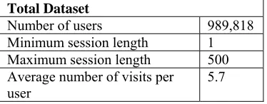
Total Dataset
Number of users 989,818
Minimum session length 1 Maximum session length 500 Average number of visits per
user 5.7
Description of the msnbc Dataset
We collected data from the UCI dataset repository (http://kdd.ics.uci.edu/) that consists of Internet Information Server (IIS) logs for msnbc.com and news-related portions of msn.com for the entire day of September 28, 1999 (Pacific Standard Time). Each sequence in the dataset corresponds to page views of a user during that twenty-four hour period. Each event in the sequence corresponds to a user’s request for a page. Requests are not recorded at the finest level of detail but they are recorded at the level of page categories as determined by the site administrator. There are 17 page categories, namely, “front page,” “ news,” “tech,” “local,” “opinion,”“on-air,” “misc,” “weather,” “health,”“living,” “business,” “sports,” “summary,”“bbs” (bulletin board service), “travel,”news,” and “msn-sports.” Fig 2 shows the characteristics of the dataset. Each page category are represented by an integer labels. For example, “frontpage”is coded as 1, “news” as 2, “tech”as 3, etc. Each row describes the hits of a single user. For example, the fourth user hits “frontpage” twice, and the second user hits “news” once and so on as shown in “Figure 1”.In the total dataset, the length of user sessions ranges from 1 to 500 and the average length of session is 5.7.[14].
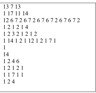
Fig 3: web navigation data with Integer lable
13 7 13 1 17 11 14
12 6 7 2 6 7 2 6 7 6 7 2 6 7 6 7 2 1 2 1 2 1 4
1 2 3 2 1 2 1 2 1 14 1 2 1 12 1 2 1 7 1 1
14 1 2 4 6 1 2 1 2 1 1 1 7 1 1 1 2 4
Fig 4: sequence representation of web navigational data
Fig 5: navigation data as a markov chain representation
S1:(0-4- 2- 8 -2 -10- 2-4-0) S2: (0-13, 13- 7, 7- 13, 13-0) S3: (0-1, 1- 17, 17- 11, 11 -14, 14-0)
(0-12,12- 6,6- 7,7- 2,2- 6,6- 7,7 -2,2 -6,6- 7,7- 6,6 -7,7- 2,2 -6,6- 7,7- 6,6- 7,7- 2,2-0)
S4: (0-1, 1- 2, 2- 1, 1- 2, 2- 1, 1- 4, 4-0) S5: (0-1, 1- 2, 2 -3, 3 -2, 2 -1, 1- 2, 1, 1 -2, 2-0)
S6: (0-1,1 -14,14- 1,1- 2,2- 1,1- 12,12- 1,1- 2,2- 1,1- 7,7- 1,1-0)
S7: (0-1, 1-0) S8: (0-14, 14-0)
S9: (0-1, 1- 2, 2- 4, 4- 6, 6-0) S10: (0-1,1-0)
S11: (0-1,1-2,2 -1,1- 6,6 -12,12 -3,3-0)
5. Conclusion
We conducted pilot experiments on msnbc data set the no of pages presented in this site are 17, so that the users can able to access only those pages [1-17], there we used a concept of grey system theory because we know the lower limit and upper limit of the page access. The page visits of the users always in sequential nature. We generated 0-13- 7- 13-0
0-1- 17- 11 -14-0
0-12- 6- 7- 2- 6- 7 -2 -6- 7- 6 -7- 2 -6- 7- 6- 7- 2-0
0-1- 2- 1- 2- 1- 4-0 0-1- 2 -3 -2 -1- 2- 1 -2-0
0-1 -14- 1- 2- 1- 12- 1- 2- 1- 7- 1-0 0-1-0
0-14-0 0-1- 2- 4- 6-0 0-1-0
markov sequences for those navigational data, then analyzed the similarity between given patternsand formed the clusters by using the proposed grey clustering algorithm. Clustering is an important task in major applications of WUM. If we want to personalize a web site the navigational data plays very important .The efficiency of the cluster is calculated by using sum of squared error. The main difference between grey relational pattern analysis and grey relational pattern analysis associated with Markov chains: In grey relational pattern analysis uses the Euclidean distance is used to find the relation between the patterns, it is possible only when the sequences are of same length. The grey relational pattern analysis associated with Markov chains finds the relation between the patterns irrespective of their lengths. Some clustering algorithms are used when the data is nonsequential in nature, but it is not possible for to capture the pair wise similarity among sequences directly, direct application of clustering algorithms without any loss of information over sequences is not possible. In terms of K-means clustering algorithm the computation of centroid of sequences is not easy, and it is difficult to perform K-means on the sequential data. The data which is in sequential nature there must exist a relation between the patterns then only it is possible to capture the pair wise similarity among sequences. The grey relational analysis is used to determining the relationships between the patterns.
References
[1] R. Kosala, H. Blockeel, Web mining research: a survey, ACM SIGKDD Explorations Newsletter 2 (1) (2000)1–15.
[2] F. M. Facca and P. L. Lanzi, "Mining interesting knowledge from web logs: a survey," Data & Knowledge Engineering, vol. 53, pp. 225-241, 2005
[3] Deng, J.L. Introduction to Grey System Theory, The journal of Grey theory, Vol. 1, Issue 1, 1988, pp. 1-24.
[4]Deng, J.L. Properties of relational space for Grey systems, In essential topics on Grey system—theory and applications, China Ocean, 1988. pp. 1-13.
[5] Bezdek, J.C.: ‘Pattern recognition with fuzzy objective function algorithm’ (Plenum Press, 1981) [6]Jain, A.K., and Dubes, R.C.: ‘Algorithms for clustering data’ (Prentice Hall, New Jersey, 1988)
[7]Gonza´lez, J., Rojas, I., Pomares, H., Ortega, J., and Prieto, A.: ‘A new clustering technique for function approximation’, IEEE Trans. NeuralNetw., 2002, 13, (1), pp. 132–142
[8]Duda, R.O., and Hart, P.E.: ‘Pattern classification and scene analysis’ (John Wiley & Sons, Inc., New York, 1973)
[9] Yeh, M.-F., Chang, J.-C., and Lu, H.-C.: ‘Unsupervised clustering algorithm via grey relational pattern analysis’, J. Chinese Grey Syst.Assoc., 2002, 5, (1), pp. 17–22
[10] Yeh, M.-F., and Wang, T.-Y.: ‘A new grey self-organizing feature map’. Proc. Joint Conf. AI, Fuzzy System, and Grey System, Taipei,Taiwan, 2003
[11] Carpenter, G.A., and Grossberg, S.: ‘A massively parallel architecture for a self-organizing neural pattern recognition machine’, Comput. Vis.Graph. Image Process., 1987, 37, (1), pp. 54–115
[12] Su, M.-C., Declaris, N., and Liu, T.-K.: ‘Application of neural network in cluster analysis’. Proc. IEEE Int. Conf. on System, Man, and Cybernetics, 1997, Vol. 1, pp. 1–6
[13] P. Kumar, R.S. Bapi, P.R. Krishna, SeqPAM: a sequence clustering algorithm for Web personalization, International Journal of Data Warehousing and Mining 3 (1) (2007) 29–53.
[14] K.-C. Chang and M.-F. Yeh," Grey relational analysis based approach for data clustering",IEE Proc.-Vis. Image Signal Process., Vol. 152, No. 2, April 2005
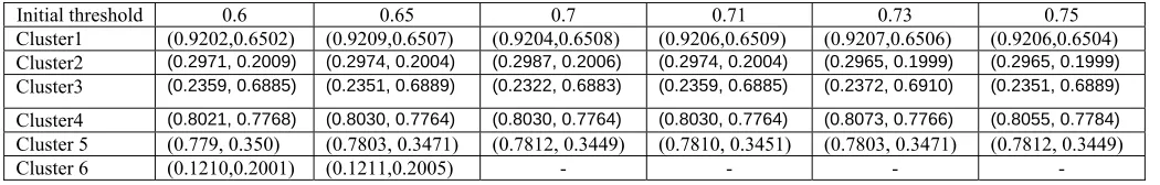
Table 1: The centroid of the clusters with threshold values
Initial threshold 0.6 0.65 0.7 0.71 0.73 0.75
Cluster1 (0.9202,0.6502) (0.9209,0.6507) (0.9204,0.6508) (0.9206,0.6509) (0.9207,0.6506) (0.9206,0.6504) Cluster2 (0.2971, 0.2009) (0.2974, 0.2004) (0.2987, 0.2006) (0.2974, 0.2004) (0.2965, 0.1999) (0.2965, 0.1999) Cluster3 (0.2359, 0.6885) (0.2351, 0.6889) (0.2322, 0.6883) (0.2359, 0.6885) (0.2372, 0.6910) (0.2351, 0.6889) Cluster4 (0.8021, 0.7768) (0.8030, 0.7764) (0.8030, 0.7764) (0.8030, 0.7764) (0.8073, 0.7766) (0.8055, 0.7784) Cluster 5 (0.779, 0.350) (0.7803, 0.3471) (0.7812, 0.3449) (0.7810, 0.3451) (0.7803, 0.3471) (0.7812, 0.3449)