The effect of model selection on cost-effectiveness research: a comparison of kidney function-based microsimulation and disease grade-based microsimulation in chronic kidney disease modeling

R E S E A R C H A R T I C L E

Open Access

The effect of model selection on

cost-effectiveness research: a comparison of

kidney function-based microsimulation and

disease grade-based microsimulation in

chronic kidney disease modeling

Shusuke Hiragi

, Hiroshi Tamura

, Rei Goto

and Tomohiro Kuroda

Abstract

Background:Cost effectiveness research is emerging in the chronic kidney disease (CKD) research field. Especially, an individual-level state transition model (microsimulation) is widely used for these researches. Some researchers set CKD grades as discrete health states, and the transition probabilities between these states were dependent on the CKD grades (disease grade-based microsimulation, MSM-dg), while others set estimated glomerular filtration rate

value which determines the severity of CKD as a main variable describing patients’ continuous status (kidney

function-based microsimulation, MSM-kf). MSM-kf seems to reflect the real world more precisely but is more difficult to implement. We compared the calculation results of these two microsimulation models to evaluate the effect of model selection on CKD cost-effectiveness analysis.

Methods: We implemented simplified MSM-dg and MSM-kf emulating natural course of CKD in general, and

compared models using parameters derived from an IgA nephropathy cohort. After checking these models’

overall behavior, life-years, utilities, and thresholds regarding intervention costs below which the intervention is thought as dominant (V0) or cost-effective (V1) were calculated. In addition, one-way and probabilistic sensitivity analyses were performed.

Results: With base-case parameters, the calculated life-years was shorter in MSM-dg (73.89 vs. 75.80 years) while the thresholds were almost equal (86.87 vs. 90.43 (V0), 132.29 vs. 146.25 [V1 in 1000 USD]) compared to MSM-kf. Sensitivity analyses showed a tendency of the MSM-dg to show shorter results in life-years. V0 and V1 were distributed by approximately ±100,000 USD (V0) and ± 150,000 USD (V1) between models.

Conclusions: Estimated cost-effectiveness thresholds by both models were not the same and its difference distributed too wide to be ignored. This result indicated that model selection in CKD cost-effectiveness research has large effect on their conclusions.

Keywords: Chronic kidney disease, Health economics, Cost effectiveness analysis, Disease modeling

* Correspondence:[email protected]

1_{Division of Medical Information Technology and Administration Planning,}

Kyoto University Hospital, 54 Kawaharacho, Shogoin, Sakyo-ku, Kyoto 606-8507, Japan

2_{Department of Nephrology, Kyoto University Hospital, 54 Kawaharacho,}

Shogoin, Sakyo-ku, Kyoto 606-8507, Japan

Full list of author information is available at the end of the article

Introduction

Chronic kidney disease (CKD), defined as impaired kidney function, is a very common disease that causes a high mortality rate and lowers quality of life (QOL) [1]. Progression of CKD to end-stage renal disease (ESRD) necessitates the renal replacement therapy (RRT, e.g. hemodialysis, peritoneal dialysis, or kidney transplant-ation), a costly [2] and lifelong treatment. As it is impos-sible to reverse renal impairment in CKD, in general, the effectiveness of management is judged by the extent to which disease progression is delayed.

CKD is said to progress gradually in a certain rate, depending on the underlying disease [3]. Various treat-ments developed to slow CKD progression have been investigated [4–6], and some researchers have evaluated the cost-effectiveness of these treatments [7–9]. One of the most utilized statistics for the measurement of cost-effectiveness is the incremental cost-effectiveness ratio (ICER), which is defined as the additional cost of a given treatment divided by the additional units of effects produced by the treatment. However, when we intend to analyze in a longer time horizon like CKD, which is lifelong disease, it is difficult to observe health utilities derived from treatments directly, because following patients for such a long time is typically not feasible.

Currently, computer simulations based on mathemat-ical modeling are utilized to emulate patients’prognoses in longer time horizon [10], and in particular, the deci-sion analytic models are widely used. When evaluating a target intervention (e.g. drug, treatment), researchers first develop a disease prognosis model using parameters such as mortality rate, disease progression speed, cost, and QOL derived from epidemiological and in vitro data [11,12]. Once the model is validated, the next step is to calculate the time courses of virtual patients using com-puter software and extract cost-effectiveness results.

In the decision analytic model, there are several ways to emulate the prognosis of a disease including decision tree analysis, and state transition modeling (STM). Decision tree analysis becomes unwieldy when many possible out-comes exist or when the follow-up period is very long [13] as with CKD. Comparably, STM is suitable for modeling

lifelong diseases because these models are relatively simple and simulations can be carried out recursively. In STM, researchers define possible discrete health states that the patient can develop and input transition probabilities

between them [14–16]. There are two types of STM:

cohort-level STM and individual-level STM (microsimula-tion). Cohort-level STM simulates the average experience of the patients in a cohort, while individual-level STM, also called as microsimulation (MSM), simulates individ-ual patient histories over time. Both STM models assume state transition occurs at once per predetermined time cycle [17].

CKD is defined by abnormalities of kidney structure or function, present for more than 3 months, with implications for health [18]. Structural abnormality is detected using urine sediment or imaging and so on, while functional abnormalities are defined by a glom-erular filtration rate (eGFR) less than 60 mL/min/ 1.73 m2

. The disease is classified into six grades accord-ing to eGFR (Table1) [18], and sometimes the severity of kidney function impairment advances from grade 5 CKD to the condition named ESRD, in which patients are dependent on RRT for survival. eGFR is considered to reflect the total capacity of body waste filtration by tiny renal components known as nephrons. Two million nephrons are thought to exist in normal kidneys, which individually lose function for various reasons such as nephritis or diabetes. Therefore, eGFR is thought to decline steadily over time, which is supported by epidemiological study [19].

STM basically assumes discrete health statuses which patients can become. Therefore, researchers have used CKD grades as discrete health states between which transition probabilities are dependent on these grades (hereinafter referred to as disease grade-based microsimulation, MSM-dg). A research group also tried to find out these transition probabil-ities between these states in general population [20]. MSM-dg is easy to implement with commercially available software, but from the clinical viewpoint, the assumption that CKD stages are discrete states and transition probabilities are constant within a certain

Table 1Glomerular filtration rate (GFR) categories in chronic kidney disease (CKD). Patients with CKD G1 and G2 have normal eGFR value and have other evidence of kidney damages (e.g. proteinuria)

GFR category GFR (mL/min/1.73 m^2) Terms

G1 ≥90 Normal or high, with evidence of kidney damage

G2 60–89 Mildly decreased, with evidence of kidney damage

G3a 45–59 Mildly to moderately decreased

G3b 30–44 Moderately to severely decreased

G4 15–29 Severely decreased

G5 < 15 Kidney failure

grade is unrealistic because severity of the disease is defined by eGFR, which is continuous variable declin-ing constantly. In contrast, STM usdeclin-ing eGFR as a constantly changing variable (hereinafter referred to as kidney function-based microsimulation, MSM-kf ) has also been implemented [21], in spite of its diffi-culty in implementation, and it seems to emulate real world more precisely. Aforementioned models are based on different assumptions; health states are discrete or continuous, and thus it is possible that they show different results for the same research topic. So far, there is no research examining the dif-ference in calculation results between these models, which can affect the conclusion of cost-effectiveness research. Hence, we aimed to compare the calculation results of these modeling methods and evaluate the effect of model selection on research conclusion to provide information for future CKD health economics investigators.

Methods

We implemented simplified MSM-dg and MSM-kf models that were not intended to describe a specific kidney disease but instead to simulate the natural course of CKD in general, for use in comparing re-sults derived from them. The details of development and the comparisons are described below.

Implementing disease grade-based microsimulation (MSM-dg)

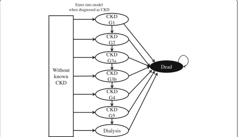
We implemented individual-level STM (microsimulation, MSM) in which we set CKD grades as health states and assumed transition probabilities between states were dependent on these grades only (Fig.1), adhering to con-ventional STM assumption. Once the kidney is damaged, the damage generally cannot be fully cured. Thus, the target population in cost-effectiveness research for treating kidney disease can be assumed to have grade 1 or more advanced CKD stages, or ESRD. With this model, the virtual cohort’s time course was computed as shown in the flowchart on Additional file1: Figure S1. Mortality rates were set as a function of age, sex, and CKD grade and that of patients in the predialysis and dialysis periods were set separately. Time cycle was set as 1/4 years based on the Japanese CKD guideline which recommends every CKD patient should be followed-up with eGFR measure-ment every 3 months [22]. In general, visiting an internal medicine clinic once every 3 months is common practice [23]. We repeated the process for each individual in the virtual cohort and acquired historical data including each individual’s health state, accumulated cost, and utility.

Implementing kidney function-based microsimulation (MSM-kf)

Next, we implemented MSM-kf in which we set only two health states (alive and dead), but the alive state has

CKD

G1

CKD

G2

CKD

G3a

CKD

G3b

CKD

G4

CKD

G5

Dialysis

Dead

Without

known

CKD

Enter into model when diagnosed as CKD

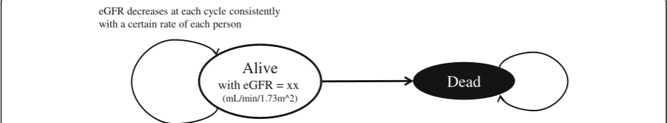
eGFR value as constantly declining variable (Fig.2). The decline rates were sometimes said to be non-linear [24], but we assumed widely-believed constant decline rate for simplicity. The transition probability between alive and dead states is dependent on CKD grades, which is determined only by the eGFR value. We assumed the de-cline rates are different by person to person. The mean and standard deviations of the rate are already well ex-amined [25–27], and we utilized these data when devel-oping our model. We assumed a log-normal distribution for the rates of eGFR decline [28], with assumption that no patient had continuously increasing eGFR value.

The simulation flowchart is shown in Additional file2: Figure S2. Mortality rates, accumulated costs, and utilities were analyzed as described for the MSM-dg implementa-tion. The conversion from eGFR to CKD grade was based on the aforementioned KDIGO definition, and we as-sumed that patients with an eGFR < 7 mL/min/1.73 m^2 were ESRD who required RRT according to the IDEAL study [29]. We also set time cycle as 1/4 years with the same reason explained in MSM-dg implementation section. The historical data of each patient was obtained using methods similar to those described for MSM-dg, and we calculated several parameters discussed below.

Parameter translation for model comparison

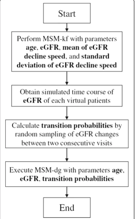
When comparing MSM-dg and MSM-kf, it is essential to translate parameters. In particular, transition probabilities in MSM-dg and eGFR decline rates in MSM-kf. Generally, previous researchers obtained the transition probabilities for MSM-dg from medical records [20,30]. That is, they compared the eGFR of patients at two visits and calcu-lated the fraction of those who proceeded to the next grade among all patients with a particular CKD grade. On the contrary, investigators applying MSM-kf used eGFR decline rates obtained from previous cohort studies [21,

31]. Therefore, we at first performed our MSM-kf with pa-rameters obtained from existing epidemiological data. Next, from the historical eGFR data acquired with the MSM-kf, we randomly sampled the grade transition be-tween two consecutive visits and estimated the transition probabilities to emulate the method described above to

acquire transition probabilities. Finally, we inputted the calculated transition probabilities for MSM-dg (Fig.3). By implementing the aforementioned translation, we could calculate transition probabilities from eGFR decline slope, resulting in comparison between MSM-dg and MSM-kf with same conditions.

Comparison of estimation results with dg and MSM-kf

We compared MSM-dg and MSM-kf to evaluate the dif-ferences in the calculation results. In this study, we set MSM-kf as reference model, considering its potential to reflect the reality more than MSM-dg. As base case ana-lysis parameters, we used data from prior epidemiological study on IgA nephropathy, a major cause of CKD [32]. Clinically, utility changes from the disease and natural course represent those of typical CKD and cost structure may be the same, suggesting the data was suitable for our purpose. The study, named VALIGA [33], consisted of pa-tients from 13 European countries. Adhering the data, we made our virtual cohort include equal numbers of 37-year old men and women with an eGFR of 76 mL/min/ 1.73 m2. Mortality rates were acquired from general popu-lation of Ontario [34–36], Canada and dialysis patients from Japan [37] due to limited available data (Detail is de-scribed in supplementary material provided as

Add-itional file 3). The study showed immunosuppressant

therapy for IgAN can slow the rate of eGFR decline from

−2.2 ± 6.5 to−1.3 ± 8.5 mL/min/1.73 m2/year. We set the

initial parameters as shown in Table 2. At first, we

checked these models’ behavior by means of

Kaplan-Meier plot of renal survival rates. Renal survival rate is a ratio of patients not requiring RRT at a point of certain time, which is common indicator in nephrology research. Afterwards, we calculated and compared unadjusted life years, discounted quality-adjusted life-years (QALYs), costs, and new parameters defined below with both MSM-dg and MSM-kf.

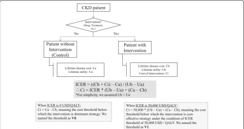
Here, we introduced two new parameters indicating cost thresholds below which an interventions of interest are dominant strategy, and cost-effective (Fig.4). In par-ticular: the maximum present value of the cost of an

Dead

Alive

with eGFR = xx

(mL/min/1.73m^2)

eGFR decreases at each cycle consistently with a certain rate of each person

intervention below which the intervention can be dom-inant over the control (named V0 in this study) under the assumption that utility increases by the intervention, and the maximum present value of the cost of an inter-vention below which the interinter-vention can be thought as cost-effective (V1). For this study, we assumed the threshold of cost-effectiveness was 50,000 USD / QALY adhering to prior literature [38]. The formulas used to calculate V0 and V1 are:

V0¼Ca−Cbðunder the assumptions o f Ub>UaÞand V1

¼50;000 ðUb−UaÞ þ ðCa−CbÞ

Where Ca = total cost of disease without intervention, Cb = total cost of disease with intervention (excluding intervention costs), Ua = total utility without interven-tion, and Ub = total utility with intervention. When Ca > Cb + cost of intervention, the intervention is dominant

over the control. Hence, V0 = Ca–Cb. When (Cb + cost of intervention–Ca) / (Ub–Ua) < 50,000, the interven-tion will be seen as cost-effective. Hence, V1 = 50,000 ×

(Ub–Ua) + (Ca–Cb).

These variables represent the value we can pay for the intervention (detail is shown in Fig.4). By calculat-ing them with MSM-dg and MSM-kf, we can evaluate the effect of modelling methods on researchers’ conclu-sion whether a new expensive intervention is cost effective or not.

Sensitivity analysis

There was unavoidable uncertainty in the parameters ex-tracted from the VALIGA cohort, which provided only

cohort-level information. Therefore, we performed

one-way sensitivity analysis to overcome this limitation. We altered eGFR (30–90 mL/min/1.73 m^2), initial age (30–60 years old), mean eGFR decline rate (0.5–10.0 mL/ min/1.73 m^2/year), standard deviation of the eGFR decline rate (0.5–10.0 mL/min/1.73 m^2/year), and other

variables listed in Table 2 and calculated difference

between estimated life years, utilities, costs, V0 and V1. Researchers may be interested in not only IgAN, but also other diseases causing CKD, in other cohorts. Thus, we also performed probabilistic sensitivity analysis of these parameters and plotted the estimated life years, utilities, costs, and V0 and V1, from both models.

We used the Numpy and Math libraries. (Source codes are provided as Additional files4and5). For visualization, we used R 3.4.2 software [39] and “survminer” package [40] to draw the Kaplan-Meier curve.

Results

Comparison of models

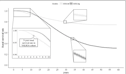
Figure 5 shows the Kaplan-Meier plot of the renal

survival rates in both models. That of 5-years follow up in VALIGA cohort was also shown in zoomed area in lower left for comparison. Renal survival rates at 5 years were 99.8% in MSM-dg, 97.8% in MSM-kf, and 97.8% in VALIGA cohort.

The estimated life-years determined using MSM-dg were 73.89 ± 12.14 years (control) and 75.80 ± 12.82 years (immunosuppressant therapy). The estimated life-years using MSM-kf were 76.35 ± 12.44 years (control) and 78.80 ± 12.62 years (immunosuppressant therapy). The ex-pected utilities (discounted) from the starting point calcu-lated by MSM-dg were 19.43 ± 4.06 QALYs (control) and 20.00 ± 4.33 QALYs (immunosuppressant therapy). The ex-pected utilities calculated by MSM-kf were 20.34 ± 4.08 QALYs (control) and 21.12 ± 4.08 QALYs (immunosup-pressant therapy). The present values of expected lifetime costs calculated by MSM-dg were 286.85 ± 350.27 thou-sand dollars (control) and 213.42 ± 365.60 thouthou-sand dollars (immunosuppressant therapy, excluding intervention costs).

The present values of expected lifetime costs calculated by MSM-kf were 199.98 ± 298.13 thousand dollars (control) and 122.99 ± 265.59 thousand dollars (immunosuppressant therapy, excluding intervention costs). The V0 values cal-culated from acquired data were 86,870 USD (MSM-dg) and 90,430 USD (MSM-kf). The V1 values calculated from the same data were 132,290 USD (MSM-dg) and

146,250 USD (MSM-kf) (Table 3). In base cases, the

MSM-dg results showed shorter life-years, lower utilities, and greater costs than MSM-kf did. As a result, MSM-dg showed smaller result in both V0 and V1 compared to MSM-kf in this circumstance.

Sensitivity analysis

The results of the one-way sensitivity analysis revealed that MSM-dg showed shorter and lower life-years and utilities than MSM-kf in most cases, respectively. Also similar to the base case analyses, the calculated costs de-termined using MSM-dg were greater by approximately 50,000–100,000 USD in most cases. The difference in V0 and V1 values did not show specific tendencies, and the differences distributed within approximately −50,000 to

100,000 USD (V0) and−100,000 to 150,000 USD (V1).

The detailed result of one-way sensitivity analyses are shown in Additional file6: Figure S3.

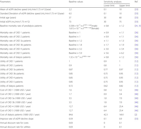
Table 2Parameters of base case and sensitivity analyses. There were no CKD 1 patients as the initial eGFR was below 90 mL/min/ 1.73 m^2. Hence, we did not perform sensitivity analyses of mortality rate, utility, and cost for CKD 1 patients

Parameters Baseline values Sensitivity analyses Ref.

Lower limit Upper limit

Mean of eGFR decline speed (mL/min/1.73 m^2/year) 2.2 0.1 10 [33]

Standard Deviation of eGFR delcline speed (mL/min/1.73 m^2/year) 6.5 0.1 10 [33]

Initial age (years) 37 30 60 [33]

Initial eGFR (mL/min/1.73 m^2) 73 30 75 [33]

Baseline mortality rate of predialysis patients 3.338 × 10−5×e0.091 ×age(male)

1.615 × 10−5_×e0.098 ×age_(female) × 0.8 × 1.2 [34,35]

Mortality rate of CKD 1 patients Baseline × 1 × 0.9 × 1.1 [36]

Mortality rate of CKD 2 patients Baseline × 1 × 0.9 × 1.1 [36]

Mortality rate of CKD 3a patients Baseline × 1.2 × 1.1 × 1.3 [36]

Mortality rate of CKD 3b patients Baseline × 1.8 × 1.7 × 1.9 [36]

Mortality rate of CKD 4 patients Baseline × 3.2 × 3.0 × 3.4 [36]

Mortality rate of CKD 5 patients Baseline × 5.9 × 5.6 × 6.2 [36]

Mortality rate of dialysis patients 1.32 × 10−3_×e0.060 ×age _{× 0.8 × 1.2 [36]}

Utility of CKD 1 patients 1 0.9 1 [12]

Utility of CKD 2 patients 0.9 0.8 1 [12]

Utility of CKD 3a patients 0.87 0.77 0.97 [12]

Utility of CKD 3b patients 0.85 0.75 0.95 [12]

Utility of CKD 4 patients 0.85 0.75 0.95 [12]

Utility of CKD 5 patients 0.85 0.75 0.95 [12]

Utility of dialysis patients 0.72 0.62 0.82 [12]

Cost of CKD 1 (1000 USD / year) 1.6 0.8 3.2 [46]

Cost of CKD 2 (1000 USD / year) 1.7 0.9 3.4 [46]

Cost of CKD 3a (1000 USD / year) 3.5 1.8 7.0 [46]

Cost of CKD 3b (1000 USD / year) 3.5 1.8 7.0 [46]

Cost of CKD 4 (1000 USD / year) 12.7 6.4 25.4 [46]

Cost of CKD 5 (1000 USD / year) 12.7 6.4 25.4 [46]

Cost of dialysis patients (1000 USD / year) 84.6 42.3 169.1 [2]

Improve rate of eGFR decline slope 0.59 0.1 0.9 [33]

Annual discount rate for costs 0.03 0 0.1

Annual discount rate for utilities 0.03 0 0.1

The probabilistic sensitivity analysis revealed that life-years and utilities calculated with MSM-dg were shorter and lower, respectively, than those with MSM-kf in approximately two thirds of parameter sets. Costs calculated with MSM-dg were greater than costs calculated with MSM-kf in two thirds of cases. Regarding V0 and V1 values, the difference between both results distributed across zero almost equally. The vast majority of results

(95%) were between −91,300 USD and 75,700 USD (V0),

and between −108,300 USD and 98,600 USD (V1). The

scatter plots of results of probabilistic sensitivity analyses are shown in Additional file7: Figure S4.

Discussions

We compared two microsimulation models of CKD that are utilized within the field of health economics research: we called them MSM-dg and MSM-kf. First, we

im-plemented simplified models. The Kaplan-Meyer

curves of calculated results declined steadily, indicat-ing that our implementations did not deviate from the reality so much.

We introduced two new parameters, V0 and V1, for our base-case settings comparison because directly analyzing cost-effectiveness of currently available therapy

has scarce meaning. That is, currently available,

partially-effective immunosuppressant therapy for IgAN [41] costs only 1200 USD [42,43], which is too inexpen-sive to analyze cost-effectiveness with commonly-applied 50,000 USD/QALY threshold. We defined V0 as the dif-ference between the total estimated costs of the control

and intervention groups excluding the intervention cost. When the disease costs of the control group exceed those of the intervention group, V0 is positive and iden-tical to the maximum present value of the cost of the intervention below which the intervention is dominant strategy over the control. Likewise, V1 represents the maximum present value of the intervention cost under the condition that the cost-effectiveness threshold is

50,000 USD/QALY. The threshold determining

cost-effectiveness is a topic of health economics research [44] but is outside the scope of this study. Current effort on drug discovery focuses on innovative and expensive ones which should be examined cost-effectiveness. It is quite possible that such an expensive drug for stopping CKD would be invented in near future. From the viewpoint of payers or societies, it is very important to estimate the threshold below which an intervention is cost-effective for future CKD interventions in the era of increasing medical costs. In this context, V0 and V1 express this threshold.

In base-case analysis, MSM-dg results showed shorter life years and QALYs, and larger costs compared to MSM-kf. V0 were 86,870 USD by MSM-dg and 90,430 USD by MSM-kf, meaning that investigators who use MSM-dg will conclude an intervention is dominant strategy when the present value of the intervention cost is below 86,870 USD while those who use MSM-kf do so if the present value is below 90,430 USD. If the actual cost is between 86,870 and 90,430USD, conclusion be-comes different due to selection of modeling method.

Likewise, if the actual cost is between 132,290 USD and 146,250 USD, investigators conclude differently about cost-effectiveness of the intervention in the condition of ICER threshold is 50,000USD / QALY. This result indi-cates that the conclusion whether an intervention is dominant strategy or cost-effective is easily changed by the selection of their modeling method. In base-case setting, investigators who use MSM-kf will conclude the intervention is cost-effective more likely than those who use MSM-dg.

Our one-way sensitivity analysis showed that MSM-dg showed shorter results in life-years (by approximately 1.5–3.0 years) and utilities compared to MSM-kf but did larger results in costs in most cases. V0 and V1 values did not show specific tendencies, but the results

calculated by MSM-dg were different from those by

MSM-kf by approximately −50,000 to 100,000 USD

(V0) and−100,000 to 150,000 USD (V1). These results

imply that even if the initial parameters were uncertain, the tendencies were applicable with regard to calculated life years, utilities, and costs. Difference in V0 and V1 distributed largely, indicating that the threshold for an intervention to be dominant or cost-effective can fluctu-ate within these margins based on the selection of mod-eling method. These fluctuation margins are three to five times greater than the GDP per capita in the United States [45]; an amount that is difficult to ignore.

We performed probabilistic sensitivity analysis for proving generalizability of our findings. The analysis showed similar results to one-way sensitivity analysis.

5-year renal survival rate in VALIGA cohort

Fig. 5Kaplan-Meier curve of renal survival rates calculated with MSM-dg and MSM-kf. The black line represents renal survival rate calculated with MSM-kf; gray line with MSM-dg. Light color bands represents 95% confidence intervals

Table 3Calculation results of base cases. Standard deviations are shown in parentheses

MSM-dg MSM-kf

Immunosuppressant therapy Control Immunosuppressant therapy Control

Life years (years) 76.35 (± 12.44) 73.89 (± 12.14) 78.80 (± 12.62) 75.80 (± 12.82)

Utility (years) 20.34 (± 4.08) 19.43 (± 4.06) 21.12 (± 4.08) 20.00 (± 4.33)

Cost (1000 USD) 199.98 (± 298.13) 286.85 (± 350.27) 122.99 (± 265.59) 213.42 (± 365.60)

V0 (1000 USD) 86.87 90.43

V1 (1000 USD) 132.29 146.25

MSM-dgDisease grade-based microsimulation,MSM-kfKidney function-based microsimulation,V0boundary below which the intervention is dominant;V1

The differences between the V0 values calculated using

MSM-dg versus MSM-kf were in the range of −91,300

USD and 75,700 USD in 95% of the results while that of

V1 values ranged from−108,300 USD and 98,600 USD.

These amounts are also difficult to ignore.

The reason for this difference can be partially ex-plained by the characteristics of MSM-dg which ignored time-dependent variety of patients within a single health

states. A cohort with eGFR of 55 mL/min/1.73m2(CKD

G3a) at the beginning of a simulation, for instance, should have time-dependent transition probabilities to G3b because the fraction of patients with eGFR close to 45 mL/min/1.73 m2 (threshold between CKD G3a and G3b) will increase as the time goes, under the assump-tion of constant eGFR decline.

Policymakers can use cost-effectiveness studies to determine whether a given intervention is worth paying for. CKD is a common and lifelong disease with treat-ments available that may slow its progression to ESRD. Based on the results of our study, MSM-dg and MSM-kf based on different health states assumptions may produce different conclusions. In particular, compared to MSM-kf, MSM-dg showed shorter or smaller results in life-years and utilities, and estimated costs. The differ-ences the between the V0 and V1 values were distributed bilaterally across zero, and the margins were relatively large. At a glance, MSM-kf emulates the real world more precisely from the clinical viewpoint. However, MSM-dg is easier to understand than MSM-kf, and it is more eas-ily implemented using commercially available software. Simulation methods cannot avoid inaccuracy, and inves-tigators must consider the biases inherent to the calcula-tion methods they utilize. Our results may help clarify the biases derived from the selection of MSM-dg or MSM-kf for future CKD cost-effectiveness researchers.

This research has several limitations. First, we ignored major parameters affecting CKD progression such as race, ethnicity, and major cardiovascular risks for simpli-city. Second, we did not consider kidney transplantation, which has a different cost structure than dialysis as RRT. Kidney transplantation is relatively inexpensive, and has become a considerable option for ESRD patients. This time we did not include kidney transplantation in our models to maintain simplicity, but it may be possible to include post-transplantation status into the models after reliable cost and utility data are accumulated. Third, we assumed constant eGFR decline rates, which is widely believed but sometimes pointed out to be incorrect. However, even when non-linear decline was assumed, our method of comparison could be applied even though it may become complicated, and similar difference would be possibly shown. Lastly, we only showed differ-ence in calculation results, but we could not definitively determine which model is superior because of limited

reliable accuracy indicators. Nevertheless, we believe this information is important.

Conclusions

MSM-dg, based on a conventional discrete state transi-tion assumptransi-tion, tends to show smaller results in util-ities and larger ones in costs compared to more-realistic MSM-kf, based on the assumption of continuous state change in CKD disease modeling. The selection of a dis-ease modelling method in cost-effectiveness researches of CKD intervention causes difficult-to-ignore fluctua-tions in their conclusions.

Additional files

Additional file 1: Figure S1.Implemented MSM-dg flowchart. Uniform random numbers were used for determination of live or death, and progression of CKD grade. Each period’s costs and utilities were added after a state transition was determined. (PPT 192 kb)

Additional file 2: Figure S2.Implemented MSM-kf flowchart. Log-normal random numbers with reported mean and standard deviation values were used as the patient’s constant eGFR decline rate. Similar to MSM-dg, a uniform random number was generated for determination of live or death. If the patient survives, his/her eGFR declined according to the previously assigned constant rate. Each period’s costs and utilities were added after a state transition was determined. (PPT 174 kb)

Additional file 3: Figure S2.Supplementary documents describing parameter determination in detail. (DOC 128 kb)

Additional file 4: Python source code for models implementation. Python source code which implements MSM-kf and MDM-dg models. (TXT 9 kb)

Additional file 5: Python source code for models comparison. Python source code which implements models comparison. Users have to modify the code to import python code provided as Additional file4 (Python source code for models implementation). (TXT 3 kb)

Additional file 6: Figure S3.a-e Results of one-way sensitivity analyses. (PPT 132 kb)

Additional file 7:Figure S4.a-e Results of probabilistic sensitivity analyses. (PPT 3755 kb)

Abbreviations

CKD:Chronic kidney disease; eGFR: Estimated glomerular filtration rate; ESRD: End-stage renal disease; ICER: Incremental cost-effectiveness ratio; IgAN: IgA nephropathy; MSM: Microsimulation; MSM-dg: Disease grade-based microsimulation; QALY: Quality-adjusted life-year; QOL: Quality of life; RRT: Renal replacement therapy; STM: State transition modelling

Acknowledgements

We would like to thank Drs. Genta Kato and Kazuya Okamoto, for their valuable advice in regard to technical and medical affairs. We gratefully acknowledge Ms. Kaori Shiomi, Yoko Hara, and Yuko Furusawa for secretarial assistance. We also thanks to Dr. Motoko Yanagita, Professor of Nephrology, graduate school of medicine, Kyoto University, for her generous advice and assistance in regard to affairs relating nephrology.

Funding

Availability of data and materials

The source codes developed during this study are available from the corresponding author on reasonable request.

Authors’contributions

SH wrote the main manuscript text and prepared figures and tables. HT supervised programming implementation. RG supervised theoretical matters. TK leaded the discussion and the team. All authors reviewed, read and approved the final manuscript.

Ethics approval and consent to participate

Not applicable. This study did not involve human participants, human data or human tissue.

Consent for publication

Not applicable. This study does not contain any individual person’s data.

Competing interests

The authors declare that they have no competing interests.

Publisher’s Note

Springer Nature remains neutral with regard to jurisdictional claims in published maps and institutional affiliations.

Author details

1_{Division of Medical Information Technology and Administration Planning,}

Kyoto University Hospital, 54 Kawaharacho, Shogoin, Sakyo-ku, Kyoto 606-8507, Japan.2Department of Nephrology, Kyoto University Hospital, 54 Kawaharacho, Shogoin, Sakyo-ku, Kyoto 606-8507, Japan.3_{Graduate School of}

Business Administration, Keio University, 2-33-28 Hiyoshi Honcho, Kohoku-ku, Yokohama, Kanagawa 223-8526, Japan.4_{Keio Business School, Keio}

University, 2-33-28 Hiyoshi Honcho, Kohoku-ku, Yokohama, Kanagawa 223-8526, Japan.

Received: 20 February 2018 Accepted: 17 October 2018

References

1. Perlman RL, Finkelstein FO, Liu L, Roys E, Kiser M, Eisele G, et al. Quality of life in chronic kidney disease (CKD): a cross-sectional analysis in the renal research institute-CKD study. Am J Kidney Dis. 2005;45:658–66.

2. Chapter 11: Medicare expenditures for persons with ESRD: UNITED STATES RENAL DATA SYSTEM. Available from:http://www.usrds.org/2015/view/v2_ 11.aspx. Cited 6 Apr 2016.

3. Part 7. Stratification of Risk for Progression of Kidney Disease and Development of Cardiovascular Disease. Am J Kidney Dis. 39:S170_–212. https://doi.org/10.1053/ajkd.2002.30946.

4. Walz G, Budde K, Mannaa M, Nurnberger J, Wanner C, Sommerer C, et al. Everolimus in patients with autosomal dominant polycystic kidney disease. N Engl J Med. 2010;363:830_–40.https://doi.org/10.1056/NEJMoa1003491. 5. Jones C, Roderick P, Harris S, Rogerson M. Decline in kidney function before

and after nephrology referral and the effect on survival in moderate to advanced chronic kidney disease. Nephrol Dial Transplant. 2006;21:2133–43. https://doi.org/10.1093/ndt/gfl198.

6. Wright JT Jr, Bakris G, Greene T, Agodoa LY, Appel LJ, Charleston J, et al. Effect of blood pressure lowering and antihypertensive drug class on progression of hypertensive kidney disease: results from the AASK trial. JAMA. 2002;288:2421_–31.

7. Mennini FS, Russo S, Marcellusi A, Quintaliani G, Fouque D. Economic effects of treatment of chronic kidney disease with low-protein diet. J Ren Nutr. 2014;24:313–21.https://doi.org/10.1053/j.jrn.2014.05.003.

8. Erickson KF, Chertow GM, Goldhaber-Fiebert JD. Cost-effectiveness of tolvaptan in autosomal dominant polycystic kidney disease. Ann Intern Med. 2013;159: 382–9.https://doi.org/10.7326/0003-4819-159-6-201309170-00004. 9. Harris A, Cooper BA, Li JJ, Bulfone L, Branley P, Collins JF, et al.

Cost-effectiveness of initiating dialysis early: a randomized controlled trial. Am J Kidney Dis. 2011;57:707–15.https://doi.org/10.1053/j.ajkd.2010.12.018. 10. Weinstein MC, O'Brien B, Hornberger J, Jackson J, Johannesson M, McCabe

C, et al. Principles of good practice for decision analytic modeling in health-care evaluation: report of the ISPOR task force on good research practices--modeling studies. Value Health. 2003;6:9–17.

11. Mazairac AH, de Wit GA, Grooteman MP, Penne EL, van der Weerd NC, den Hoedt CH, et al. Effect of hemodiafiltration on quality of life over time. Clin J Am Soc Nephrol. 2013;8:82–9.https://doi.org/10.2215/cjn.00010112. 12. Gorodetskaya I, Zenios S, McCulloch CE, Bostrom A, Hsu CY, Bindman AB, et al.

Health-related quality of life and estimates of utility in chronic kidney disease. Kidney Int. 2005;68:2801–8.https://doi.org/10.1111/j.1523-1755.2005.00752.x. 13. Drummond MFSM, Claxton K, Stoddart GL, Torrance GW. Economic

evaluation using decision-analytic modelling. Methods for the economic evaluation of health care Programmes. Oxford: Oxford University Press; 2015. p. 311_–51.

14. Sonnenberg FA, Beck JR. Markov models in medical decision making: a practical guide. Med Decis Making. 1993;13:322–38.https://doi.org/10.1177/ 0272989x9301300409.

15. Siebert U, Alagoz O, Bayoumi AM, Jahn B, Owens DK, Cohen DJ, et al. State-transition modeling: a report of the ISPOR-SMDM modeling good research practices task Force-3. Med Decis Making. 2012;32:690–700.https://doi.org/ 10.1177/0272989x12455463.

16. Briggs A, Sculpher M. An introduction to Markov modelling for economic evaluation. PharmacoEconomics. 1998;13:397–409.

17. Heeg BM, Damen J, Buskens E, Caleo S, de Charro F, van Hout BA. Modelling approaches: the case of schizophrenia. PharmacoEconomics. 2008;26:633–48.

18. Chapter 1: Definition and classification of CKD. Kidney Int Suppl. 2013;3:19– 62.https://doi.org/10.1038/kisup.2012.64.

19. Mitch WE, Walser M, Buffington GA, Lemann J Jr. A simple method of estimating progression of chronic renal failure. Lancet (London, England). 1976;2:1326_–8.

20. Luo L, Small D, Stewart WF, Roy JA. Methods for estimating kidney disease stage transition probabilities using electronic medical records. EGEMS (Washington, DC). 2013;1:1040.https://doi.org/10.13063/2327-9214.1040. 21. Hoerger TJ, Wittenborn JS, Segel JE, Burrows NR, Imai K, Eggers P, et al. A

health policy model of CKD: 1. Model construction, assumptions, and validation of health consequences. Am J Kidney Dis. 2010;55:452–62.https:// doi.org/10.1053/j.ajkd.2009.11.016.

22. Japan nephrology s. Special issue: clinical practice guidebook for diagnosis and treatment of chronic kidney disease 2012. Nihon Jinzo Gakkai shi. 2012; 54:1034_–191.

23. Schwartz LM, Woloshin S, Wasson JH, Renfrew RA, Welch HG. Setting the revisit interval in primary care. J Gen Intern Med. 1999;14:230–5. 24. Skupien J, Warram JH, Smiles AM, Stanton RC, Krolewski AS. Patterns of

estimated glomerular filtration rate decline leading to end-stage renal disease in type 1 diabetes. Diabetes Care. 2016;39:2262–9.https://doi.org/10. 2337/dc16-0950.

25. Glassock RJ, Winearls C. Ageing and the glomerular filtration rate: truths and consequences. Trans Am Clin Climatol Assoc. 2009;120:419–28.

26. Imai E, Horio M, Yamagata K, Iseki K, Hara S, Ura N, et al. Slower decline of glomerular filtration rate in the Japanese general population: a longitudinal 10-year follow-up study. Hypertens Res. 2008;31:433–41.https://doi.org/10. 1291/hypres.31.433.

27. Bartosik LP, Lajoie G, Sugar L, Cattran DC. Predicting progression in IgA nephropathy. Am J Kidney Dis. 2001;38:728–35.https://doi.org/10.1053/ajkd. 2001.27689.

28. Skupien J, Warram JH, Smiles AM, Niewczas MA, Gohda T, Pezzolesi MG, et al. The early decline in renal function in patients with type 1 diabetes and proteinuria predicts the risk of end-stage renal disease. Kidney Int. 2012;82: 589_–97.https://doi.org/10.1038/ki.2012.189.

29. Cooper BA, Branley P, Bulfone L, Collins JF, Craig JC, Fraenkel MB, et al. A randomized, controlled trial of early versus late initiation of dialysis. N Engl J Med. 2010;363:609_–19.https://doi.org/10.1056/NEJMoa1000552.

30. Blanchette CM, Liang C, Lubeck DP, Newsome B, Rossetti S, Gu X, et al. Progression of autosomal dominant kidney disease: measurement of the stage transitions of chronic kidney disease. Drugs Context. 2015;4:212275. https://doi.org/10.7573/dic.212275.

31. Orlando LA, Belasco EJ, Patel UD, Matchar DB. The chronic kidney disease model: a general purpose model of disease progression and treatment. BMC Med Inform Decis Mak. 2011;11:41.https://doi.org/10.1186/1472-6947-11-41. 32. Chapter 10: Immunoglobulin A nephropathy. Kidney Int Suppl. 2012;2:209–

17.https://doi.org/10.1038/kisup.2012.23.

34. Table 1a Complete life table, males, Ontario, Canada, 2009 to 2011: statistics Canada. Available from:http://www.statcan.gc.ca/pub/84-537-x/2013005/tbl/ tbl7a-eng.htm. Cited 16 Mar 2016.

35. Table 1a Complete life table, females, Ontario, Canada, 2009 to 2011: statistics Canada. Available from:http://www.statcan.gc.ca/pub/84-537-x/ 2013005/tbl/tbl7b-eng.htm. Cited 16 Mar 2016.

36. Go AS, Chertow GM, Fan D, McCulloch CE, Hsu CY. Chronic kidney disease and the risks of death, cardiovascular events, and hospitalization. N Engl J Med. 2004;351:1296–305.https://doi.org/10.1056/NEJMoa041031. 37. Distribution of cause of death in dialysis patients who died in 2014 stratified

by age group (in Japanese): the Japanese Society of Dialysis Therapy. Available from:http://docs.jsdt.or.jp/overview/index2014.html. Cited 19 Mar 2016. 38. Hirth RA, Chernew ME, Miller E, Fendrick AM, Weissert WG. Willingness to

pay for a quality-adjusted life year: in search of a standard. Med Decis Making. 2000;20:332–42.https://doi.org/10.1177/0272989x0002000310. 39. Team RC. A language and environment for statistical computing. Vienna: R

Foundation for Statistical Computing; 2015.

40. Kassambara A, Kosinski M, Biecek P, Fabian S. Drawing survival curves using ‘ggplot2’. 2017.http://www.sthda.com/english/rpkgs/survminer/. 41. Pozzi C, Andrulli S, Del Vecchio L, Melis P, Fogazzi GB, Altieri P, et al.

Corticosteroid effectiveness in IgA nephropathy: long-term results of a randomized, controlled trial. J Am Soc Nephrol. 2004;15:157_–63. 42. Drugbank Version 5.0. Available from:https://www.drugbank.ca/. Cited 26

Dec 2016.

43. Canada’s health expenditure: Spending on prescribed drugs increases, total growth remains slow: Canadian Institute for Health Information; 2016. Available from:https://secure.cihi.ca/estore/productFamily.htm?locale=en&pf=PFC3333. Cited 26 Dec 2016.

44. Marseille E, Larson B, Kazi DS, Kahn JG, Rosen S. Thresholds for the cost-effectiveness of interventions: alternative approaches. Bull World Health Organ. 2015;93:118–24.https://doi.org/10.2471/blt.14.138206. 45. Indicators: The World Bank. Available from:http://data.worldbank.org/

indicator/. Cited 11 Oct 2016.