The rôle of Lattice Dynamics in determining the
Griinesien Parameter and Diffusion Processes in
Minerals and their Analogues.
Nicole Ludmila Vodadlo
Department of Geological Sciences, University College London.
Submitted fo r the degree o f Doctor o f Philosophy, University o f London.
ProQ uest Number: 10106708
All rights reserved
INFORMATION TO ALL U SE R S
The quality of this reproduction is d ep en d en t upon the quality of the copy subm itted. In the unlikely even t that the author did not sen d a com plete manuscript and there are m issing p a g e s, th e se will be noted. Also, if material had to be rem oved,
a note will indicate the deletion.
uest.
ProQ uest 10106708
Published by ProQ uest LLC(2016). Copyright of the Dissertation is held by the Author. All rights reserved.
This work is protected against unauthorized copying under Title 17, United S ta tes C ode. Microform Edition © ProQ uest LLC.
ProQ uest LLC
789 East E isenhow er Parkway P.O. Box 1346
Abstract.
The determination of the structural and rheological properties of the Earth’s deep interior is severely hindered by its inaccessibility and the limitations on experimental techniques. With continuing progress being made in the development of increasingly powerful supercomputers, it is now possible to probe the Earth’s interior via predictions based upon the atomistic simulation of Earth forming minerals. It is this consolidation between the microscopic and macroscopic nature of matter that is the essence of these computer simulations, and as such make computer modelling an extremely powerful tool with which to explore the innermost parts of our planet. This thesis uses such simulation techniques to investigate the Griineisen parameter and diffusion processes in Earth forming structures.
The Griineisen parameter relates relevant thermodynamic properties and has an approximately constant, dimensionless value for most minerals over the entire pressure-temperature range for the deep interior. Its original definition is in terms of the vibrational spectrum which makes it an ideal quantity to investigate through lattice dynamics. It is this link between microscopic and macroscopic definitions of the Griineisen parameter that is investigated in this thesis.
energies and pre-exponential factors.
Acknowledgements.
To my greatest friend, MJG, and to my greatest, AJD.
I would like to thank Dr. Steve Parker for the use of his PARAPOCS computer code, and for the time and invaluable assistance both he and Dr. Alison Wall gave me during my time in Bath, along with the members of their exceptionally welcoming and accommodating group.
Within the Crystallography and Mineral Physics unit here at UCL there arc many by whom I was cerebrally challenged, especially Ian, Ross, Nancy, Monica and Chris. I would also like to thank Stan for his support and encouragement throughout. My humour has been continually uplifted by my two great friends Tim and Phillip, and my mental gymnastics will never recover from the great insights into life and the universe given to me by Atul.
Finally, I would like to thank The Professor (good heavens), my all-encompassing- scientific-guru {AESG)\ He has made my time here at UCL deeply splendid, picking me up when I have fallen, and raising me higher when I thought I had reached the pinnacle. He is a true kindred spirit, and I am greatly indebted to him.
Contents.
Abstract
Acknowledgements
Chapter 1: Introduction. 16
1.1 Introduction 16
1.2 What is Certain 17
1.3 Whole Earth Models 18
1.4 The Evolutionary Evidence 19
1.5 Seismology and the Preliminary Reference Earth Model 23
15.1 Introduction 23
1 5 2 The Derivation o f Seismic Velocities 25 1 5 3 Free Oscillations o f the Earth 26 15.4 The Preliminary Reference Earth Model 26
1 5 5 The Velocity-Depth Profile 26
15.6 The Pressure-Depth Profile 30
15.7 Seismic Tomography 31
1.6 The Thermal Model 36
1.6.1 Introduction 36
1.62 Heat Sources 37
1.63 Heat Transfer 38
1.6.4 The Adiabatic Temperature Gradient and the Geotherm 40
1.7 Mineralogical Models 41
1.8 Computer Simulation 47
1.9 The Rôle of Lattice Dynamics in Deep Earth Research 48
1.9.1 Introduction 48
1.92 The Griineisen Parameter 48
1.93 The Diffusion Coefficient 49
Chapter 2: The Computer Simulation of Solids. 52
2.1 Introduction 52
2.2 Interatomic Pair Potential Energy Functions 53
22.1 Introduction 53
2 2 2 Short Range Interactions 55
2 2 3 The Ewald Summation 59
2.3 The Total Energy within a Crystalline System 60
2.4 Static Lattice Simulation 62
2.4.1 Introduction 62
2.42 Constant Volume Minimisation 64
2.43 Constant Pressure Minimisation 65
2.5 Dynamic Simulation 69
23.1 Introduction 69
2 3 2 The Dynamical Matrix 70
23.3 Brillouin Zone Sampling 72
23.4 Thermodynamic Properties from the Frequency Spectrum 72
2.6 The Defective Lattice 75
2.6.1 Embedded Defect Simulations 76
2.62 The Supercell Method 78
2.7 The PARAPOCS Computer Code 80
2.8 Summary 83
C hapter 3: The Griineisen Param eter. 84
3.1 Introduction 84
3.2 Definitions of the Griineisen Parameter 85
3.3 Approximate Formulations of the Griineisen Parameter 91
3.4 Computer Modelling 98
3.5 Potential Models 99
3.6 Calculations on a Simple Cubic Lattice. 100
3.6.1 Short Range Pairwise Interactions 100 3.62 Long Range Pairwise Interactions 102
3.8 Summary 110
C hapter 4: The Phenomenological Approach to Diffusion in Solids 111
4.1 Introduction 111
4.2 Experimental Observations 113
4.3 Point Defects 116
4.4 The Atomic Theory of Diffusion 118
4.4.1 Vacancy Diffusion 118
4.42 Self-Diffusion 121
4.5 The Phenomenological Approach to the Calculation of AH^ for
Vacancy Diffusion 123
45.1 Introduction 123
4 5 2 Formulations o f the Debye Temperature 124 4 5 3 Calculation o f the Debye Temperatures and AH„ 129
4.6 The Pre-exponential Factor 132
4.6.1 Zener's Theory o f Vacancy Diffusion fo r Obtaining D f 132 4.6.2 Graphical Determination o f D f 134
4.7 Summary 137
Chapter 5: Computer Calculations for Absolute Ionic Diffusion in MgO
using the Supercell Method. 139
5.1 Introduction 139
5.2 Vineyard Theory 142
5.3 Potential Models 144
5.4 Sampling Techniques 145
5.5 Supercell Size 146
5.6 Schottky Defect Formation 148
5.7 Ion Migration 149
5.8 The Attempt Frequency 164
5.9 The Pre-exponential Correction Factor and the Extrinsic
Diffusion Coefficient 165
5.11 Absolute Ionic Diffusion in Magnesium Oxide 171
5.12 Summary 176
Chapter 6: Conclusions. 177
References 179
Appendices 186
A l: Proof that fo r an harmonic potential, dKldP=l 186 A2: Choosing parameters A and B fo r the Lennard-Jones potential 189 A3: Equivalence o f the Lennard-Jones and harmonic spring potential 191 A4: Proof that fo r a Lennard-Jones potential at P=0,
dKldP=(m+n+6)l3 193
A3: Choosing parameters for the Morse potential 195 A6: Constant pressure/constant volume interchange 200
List of Tables.
C hapter 1: Introduction.
1.1 Simple Earth model based on cosmic abundances 22
1.2 Summary of Earth structure 30
C hapter 3: The Grüneisen Param eter.
3.1 Comparison of various approximations to y with lattice dynamical y
(cut-off 1.3 lattice units) 102
3.2 Comparison of various approximations to y with lattice dynamical y
(cut-off 15.0 lattice units) 103
3.3 The variation of increasing y with dK/dP and dG/dP for NaCl type
structures with varying Buckingham potential parameters A and B 106
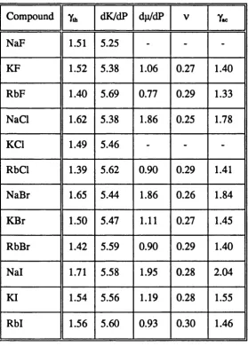
3.4 The variation of y with dK/dP and dO/dP for real materials 108
C hapter 4: The Phenomenological Approach to Diffusion in Solids.
4.1 Various Debye temperatures for simple mineral analogues 729 4.2 Debye-Waller factors and the calculated Debye temperatures 130
4.3 AHg, activation energies for atomic migration 131
4.4 p vs. T 135
4.5 p/po vs. TyT„ 136
C hapter 5: Computer Calculations for Absolute Ionic Diffusion in MgO using the Supercell Method.
5.1 The effect of supercell size 146
5.2 Schottky formation parameters for MgO 149
5.3 Bifurcation of the magnesium saddle surface 154
5.4 Bifurcation of the oxygen saddle surface 154
5.5 Results for magnesium 157
5.6 Results for oxygen 162
List of Figures.
C hapter 1: Introduction.
1.1 The interdependence of Earth models 19
1.2 Chondritic Earth model composition 21
1.3 Body wave nomenclature 24
1.4 Preliminary Reference Earth Model for mantle and core 28
1.5 Layered structure of the Earth 29
1.6 PREM velocity-depth profile 32
1.7 PREM pressure-depth profile 32
1.8 PREM Poisson’s ratio-depth profile 32
1.9 Interior of the Earth via seismic tomography 35
1.10 Convective instability of a fluid sheet heated from below 39
1.11 Current geothermal models 42
1.12 High pressure phases of the major Earth-forming minerals 44
1.13 Isotheimal phase diagram for the (MgfeiSiOg system 45
1.14 Isothermal phase diagram for the (MgfejSizO^ system 46
C hapter 2: The Computer Simulation of Solids.
2.1 Interatomic potential energy function 54
2.2 The shell model 58
2.3 Lattice vibrational frequencies as a function of wave vector 72
2.4 The Mott-Littleton embedded defect model 77
2.5 The supercell model 79
2.6 Flow diagram for PARAPOCS methodology 82
C hapter 3: The Grüneisen Parameter.
3.1 Comparison of various approximations to y with lattice dynamical y
(cut-off 1.3 lattice units) 101
3.2 Comparison of various approximations to y with lattice dynamical y
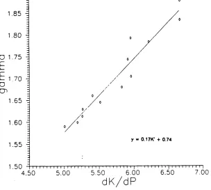
3.3 y vs. dK/dP for NaCl type structures 107
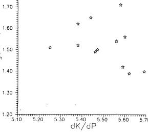
3.4 y vs. dp/dP for NaCl type structures 107
3.5 y vs. dK/dP for real materials 109
3.6 y vs. dp/dP for real materials 109
Chapter 4: The Phenomenological Approach to Diffusion in Solids.
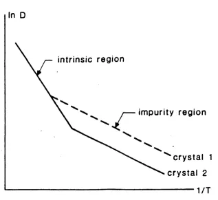
4.1 Typical experimental diffusion graph 114
4.2 Observed intrinsic and extrinsic régimes from diffusion experiments 114
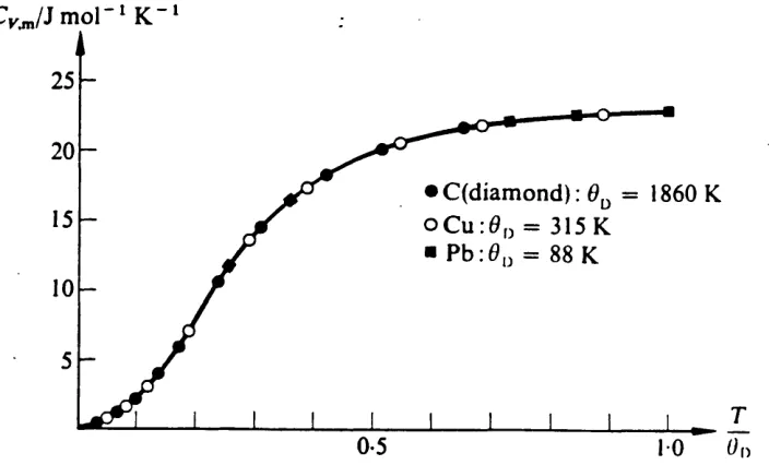
4.3 Heat capacity curve for several metals 126
Chapter 5: Computer Calculations for Absolute Ionic Diffusion in MgO using the Supercell Method.
5.1 Energy barrier for migrating defect 140
5.2 Free energy vs. cell size for both Schottky defect formation
and cation migration 147
5.3 Free energy vs. temperature for Schottky defect formation 150
5.4 Formation volume vs. temperature for Schottky defect formation 151
5.5 Formation entropy vs. temperature for Schottky defect formation 152
5.6 Bifurcation of the magnesium saddle surface 155
5.7 Bifurcation of the oxygen saddle surface 156
5.8 Migration Direction for Ionic Diffusion 158
5.9 Free energy vs. temperature for ionic migration 159
5.10 Activation volume vs. temperature for ionic migration 160
5.11 Activation entropy vs. temperature for ionic migration 161
5.12 Anharmonicity of saddle surface for magnesium 166
5.13 Anharmonicity of saddle surface for oxygen 167
5.14 Pre-exponential correction factors for magnesium and oxygen 168
5.15 Comparative extrinsic diffusion coefficients 172
5.16 Calculated absolute magnesium diffusion compared with
experimental data 174
1. Introduction.
1.1 Introduction.
The Earth is in a state of continual evolution. As residents on this planet, we are only able to observe a snapshot of her progress through the universe, and this privileged view is severely limited by our perceptions of nature; these in turn are governed by our experiences, social background and academic education, which, although sufficient for our immediate vicinity, may provide an inadequate foundation upon which to assess the true nature of reality. However, we have each been endowed with an enquiring mind and it is the wish of some to pursue such an enquiry into the very depths of our planet, regardless of our limited experience and restricted understanding. It is an instinctive trait of our character to search and research into the unknown as the story of existence unfolds before us giving way to apparantly more complex and intellectually demanding "laws" of physics which we hope will eventually give way to the underlying simplicity of Nature. Each individual may play a very small and arguably esoteric part in the game, but every piece of information gathered, whether validating or disproving current theories, adds to the enormous data base that is our current understanding of the Earth.
1.2 What is certain?
The only certainties concerning our planet arise directly from measurements taken at its surface. Any inferences made subsequently are pure supposition, albeit educated. Listed below are some examples of measurements which can be made from the surface of the Earth that are significant to its interior:
(a) mass of the Earth: 5.974xl0^kg
(b) mean radius of the Earth: 6371km
(c) average density of the Earth: 5515gcm^
(d) moment of inertia of the Earth: 0.33MR^
(e) average acceleration due to gravity at the surface: 9.8ms'^
(f) compositions of surface material: primarily water and silicate rocks
(g) densities of surface rock: 2.7-3.3gcm'^
(h) seismic wave velocities reaching the surface: 4-8kms'^
(i) free oscillation data
(j) surface temperature: 250-320K
(k) heat flux through the Earth’s surface: 4xl&^W
(1) geomagnetic field strength variations at the surface: 20,000nT-70,000nT
(m) atmospheric pressure: lOOOmbar
1.3 Whole Earth Models.
The Earth is assumed to be essentially spherically symmetric, consisting of concentric layers within the crust, mantle and core (see section 1 ^ 5 ) . The major uncertainties concerning the Earth involve its bulk properties. Is the mantle chemically homogeneous or heterogeneous? Is there layered or whole mantle convection? What are the heat sources driving mantle plumes which result in plate tectonics? What is the nature of the observed seismic discontinuities? Are the transition regions chemically controlled, phase controlled or both? What is the exact mineralogy at depth? What are the energy sources? How is the magnetic field generated?
Whole Earth models attempt to answer these problems and are usually separated into three categories: the seismological model, the thermal model and the mineralogical or
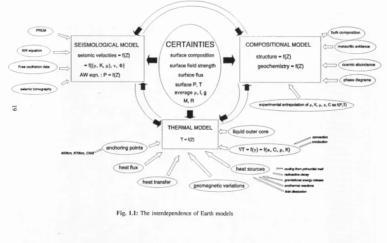
compositional model. However, the three are intimately associated and one cannot be individually discussed in isolation, since each provide mutual boundary conditions. The velocities of seismic waves arriving at the Earth’s surface are directly related to the elastic constants and density of the material through which they have passed, and therefore to the composition. The phase of the mineralogical assemblage at any depth is dependent on the local pressure and temperature, and hence to both the seismological and thermal profiles. The thermal model is constrained initially by a knowledge of the composition of the liquid iron alloy which makes up the outer core, the state of which has been inferred from the seismological profile; it is also heavily constrained by the heat flux through the Earth’s surface. This interweaving of physical properties throughout the Earth’s deep interior is illustrated by Fig. 1.1.
AW equation y c
Free osdllation data
SEISMOLOGICAL MODEL / C E R T A I N T I E ^ COMPOSITIONAL MODEL
seismic velocities - f(Z)
à m surface composition structure - f(Z)
" l((p . K. P). V, <b] surface field strength geochemistry - f(Z)
AW eqn. : P - f(Z) surface flux i
bulk composition
eelsmic tomography
I ( ^ ^ M m l c a b u n d a r ^ ^
I d l a g r ^ w ^
VO
4û0fcm, gTOhn, CMB^
average
expérimental extrapolatkxi of p. K, p, a, C as
THERMAL MODEL
(= ] C liquid outer core T-f(Z)
f(Y) - f(«. C. p.
eat sources ^ (æ ^ o rin g points
(^ ^ a t flux
heat transfer
C j ^ m a g n e tl c variations
oooing gvm prtmofdU mtH
m M oacthm O m siy
praveaflbrW eoerpy rw«Mee •xoltmmM/fmacHon»
tdÊ/amripaHon
1.4 The Evolutionary Evidence.
To understand the Earth in its present form, it is useful to have some indication of its origins. The disciplines of astronomy and astrophysics have led to a number of evolutionary models. It is generally assumed that the Sun formed through the accretion of matter after a supernova explosion (Safronov, 1972). What is more questionable is whether or not the Earth was formed at the same time, accreting out of the solar nebula, or some time later either from solar material or from other nebulous matter such as an interstellar cloud (McCrea, 1963). Whichever model is adopted, all suggest an initially hot, partially molten, undifferentiated Earth that has subsequently cooled and fractionated, losing the volatiles that are characteristic of the outer gaseous planets.
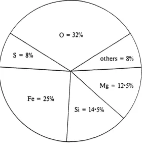
A similar history may be responsible for the characteristics of some meteorites which play a very important role in the determination of the composition of the interior Earth. Meteorites landing on the Earth’s surface are either pieces of material ripped from a much larger planetesimal, or matter that condensed out of the original solar nebula. The latter are termed chondrites and are thought to represent the most primative of all meteorites, with relative atomic abundances close to those of the Sun, removed of volatiles (Trimble, 1975). As such they are thought to be an indication of the composition of the Earth, or a part thereof, under the assumption that the Earth too formed from the solar nebula in a similar manner. Here, therefore, is one of the many pieces of evidence that suggest that the Earth, following a chondritic Earth model, has a bulk compostion shown in Fig. 12.
0 = 32%
S = 8%
others = 8
Mg = 12*5% Fe = 25%
Si = 14*5%
Table 1.1: Simple Earth model based on cosmic abundances.
Oxides Molecules Molecular Weight
Grams Weight
Fraction
MgO 1.06 40 42.4 0.250
SiOz 1.00 60 60.0 0.354
A l A 0.0425 102 4.35 0.026
CaO 0.0625 56 3.5 0.021
NagO 0.03 62 1.84 0.011
Fe^O 0.45 128 57.6 0.339
Total 169.7 1.001
It is plausible that iron is the major component of the Earth's core, in addition to some nickel; the density and moment of inertia of the Earth suggest that it is alloyed with some lighter element, of which suitable candidates are carbon, silicon, oxygen or silicon due to their relatively high abundance. The mantle is likely to be composed mainly of refractory iron poor magnesium silicates and oxides with the more volatile minerals forming hydrates, carbonates and sulphides (containing many minor elements) towards the surface.
1.5 Seismology and the Preliminary Reference Earth Model.
7.5.7 Introduction,
Seismology is the only discipline that can be used to access directly the Earth's deep interior. Analysis of the passage of seismic waves through the body of the Earth is of fundamental importance in determining how the density varies with depth. However, the first clue to compositional heterogeneity comes from the average density of surface rocks, which is far lower than that of the Earth as a whole. For a homogeneous composition, there would therefore have to be a significant amount of gravitational compression in order to account for this density variation. Simple self-compression models (Williamson and Adams, 1923) show that a chemically homogeneous Earth is highly unlikely and only a concentration near the Earth's centre of materials of considerably greater density could account for the observed whole Earth average density. To corroborate this increase in density, the observed moment of inertia, determined from the Earth's shape and precession measurements, is lower than that predicted for a homogeneous model, indicative that there is indeed a mass concentration towards the centre. To investigate this heterogeneity necessitates a density depth-profile which can be obtained from the analysis of the travel times of seismic waves as they propagate throughout the Earth after an earthquake.
Seismic or shock waves are generated through the release of stored elastic energy. This generally occurs at plate boundaries when lithospheric stresses result in brittle failure. Some of these seismic waves propagate throughout the Earth, while others propagate over its surface. The waves travelling over the surface are of two types called Raleigh waves and Love waves; while those travelling through the body of the Earth are called P-waves and S-waveSy the former longitudinal waves arriving first at a station, hence primary^ followed by the latter transverse waves, hence secondary.
oc us
s h s /
rr
SNP, \ /
I n n e f \\ core K .
r r r
F l u i d o u t e r c o r e
S K K h
S o l i d m a n : le
y '?.y.
Accurate travel time curves have been obtained through controlled underground explosions, analogous to an earthquake, which also generate seismic waves (Jeffreys and Bullen, 1940). In these experiments, the exact time of the explosion, location and depth of the focus are known, eliminating major uncertainties occuiring in the production of travel-time curves from natural earthquakes. However, earthquakes only occur in seismic zones and the stations themselves are largely restricted to continental areas, which account for only one fifth of the entire surface so such travel-times may not give information representative of the entire Earth. Nevertheless, an initial seismological profîle may be constructed in these selected areas. More recently seismic tomography has been developed to give a three dimensional representation of the structure to the Earth (see section 15.7).
1,52 The Derivation of Seismic Velocities,
Both P and S waves are elastic waves and their velocities, Vp and Vj, are given by the ratio of the elastic modulus associated with the particular deformation to density:
Vp =
(1.1)
F / = (1.2)
* P
A transverse S-wave involves the pure shear of the medium so p is just the modulus of rigidity. The passage of the P-wave, however, involves compressions and dilations of the medium which themselves subject the material to lateral constraint. So the elastic modulus required is related to the bulk modulus, K, also.
data via the relation:
F / - ^ (1.3)
' 3 * p
Adiabatic elastic moduli must be used in these equations since thermal diffusion associated with a seismic compression or rarefaction is too slow to dissipate temperature changes incurred. Equations (1.1), (12) and (1.3) illustrate how a knowledge of the seismic profile can also lead to a density profile and an elastic profile.
1.53 Free Oscillations o f the Earth.
With the occurrence of a suitably large earthquake, the Earth may be set into free oscillation, like the ringing of a bell. These vibrations result from standing waves set up by the reflections of "giant” surface waves off boundaries within the Earth and may last for several days. The wavelengths are comparable to the Earth's radius so their amplitude falls off slowly with depth making them very useful in determining elastic moduli as far down as the inner core. Here lies a totally independent method of observing interior profiles which is therefore complementary to the seismology of body waves and also useful in verification of elastic properties of the Earth's interior.
1.5.4 The Preliminary Reference Earth Model.
summary travel times, 100 normal mode Q values, (the Q-value is the quality factor^
a dimensionless measure of the dissipation a body wave) and allowed for 2-4% transverse isotropy in the upper 220km of the mantle. In doing so they managed to satisfy the entire gross Earth data set. This model has been named the Preliminary Reference Earth Model and is the most comprehensive one-dimensional description of the elastic properties of the Earth to date. The data set is fitted to a model containing 13 radial sub-divisions and 105 parameters, 13 of which are boundary parameters. Included in the model are radial distributions of density, body wave velocities, quality factors of rigidity, bulk modulus and compressional waves, the seismic parameter, the isotropic bulk modulus, rigidity, Poisson’s ratio, the gravity value, pressure and the first derivative of incompressibility with respect to pressure.(see Fig. 1.4).
1,5,5 The Velocity-Depth Profile,
Seismic inversion has shown the Earth to be of an approximately spherically symmertric structure which is layered according to the seismic discontinuities as shown in Fig. 7 J . The PREM seismic velocity-depth profile which defines these boundaries is shown in Fig. 1.6 (Dziewonski and Anderson, 1981). The principal discontinuities occur at depths of 10-50,4(X), 670,2890 and 5150km. These define the boundaries between the crust, upper mantle, transition zone, lower mantle, outer and inner core.
N) oo
z
r P P "p «'j * K P I z P p ‘ s * K M g
24 4 6346 6 3.38 8.11 4.49 38.9 1315 682 0.28 984 2571 3800 1173 5.41 13.48 7.19 112.7 6095 2794 0.30 1031 40 6331 11.2 3.38 8.11 4.48 38.8 1311 680 0.28 984 2671 3700 1230 5 46 13.60 7.23 115.1 6279 2855 0.30 1041 60 6311 17.9 3.38 8.09 4.48 38.7 1307 677 0.28 985 2771 3600 1287 5.51 13.67 7.27 117.0 6440 2907 0 .30 1052 80 6291 24.5 3.37 8.08 4.47 38.6 1303 674 0.28 986 2871 3500 1346 5.56 13.71 7.26 117.6 6537 2933 0.30 1065 IIS 6256 36.2 3.37 8.03 4.44 38.2 1287 665 0.28 988 2891 3480 13581 5.47 13.72 7.26 117.8 6556 2938 0.31 1068 185 6186 59.4 3.36 8.01 4.43 38.0 1278 660 0.28 989 2891 3480 13581 9.90 8.06 0 65.0 6441 0 0.5 1068 220 6151 71.1 3.36 7.99 4.42 37.8 1270 656 0.28 990 2971 3400 1442 10.02 8.19 0 67.2 6743 0 0.5 1051 220 6151 71.1 3.44 8.56 4.64 44.5 1529 741 0.29 990 3071 3300 1547 10.18 8.36 0 69.9 7116 0 0.5 1028 265 6106 86.5 3.42 8.65 4.68 45.6 1579 757 0.29 992 3171 3200 1651 10.33 8.51 0 72.5 7484 0 0.5 1005 310 6061 102 3.49 8.73 4.71 46.7 1630 773 0.30 994 3271 3100 1754 10.47 8.66 0 75.0 7846 0 0.5 981 355 6016 118 3.52 8.81 4.74 47.8 1682 790 0.30 995 3371 3000 1856 10.60 8.80 0 77.4 . 8202 0 0.5 956 400 597! 134 3.54 8.91 4.77 49.0 1735 806 0.30 997 3471 2900 1957 10.73 8 9 3 0 79.7 8550 0 0.5 930 400 5971 134 3.72 9.13 4.93 51.0 1899 906 0.29 997 3571 2800 2056 10.85 9.05 0 81.9 8889 0 0.5 904 450 5921 152 3.79 9.39 5.08 53.8 2037 977 0.29 998 3671 2700 2153 10.97 9.17 0 84.0 9220 0 0.5 877 500 5871 171 3.85 9.65 5.22 56.7 2181 1051 0.29 999 3771 2600 2248 11.08 9.28 0 86.1 9542 0 0 5 850 550 5821 191 39 1 9.90 5.37 5 9 6 2332 1128 0 29 1000 3871 25tlO 2342 11 19 9 18 0 88.1 9855 0 0 5 822 600 5771 210 3.98 10.16 5.51 62.6 2489 1210 0.29 1000 3971 2400 2342 11.29 9.48 0 90.0 10158 0 0.5 794 635 5736 224 3.98 10.21 5.54 63.3 2523 1224 0.29 1001 4071 2%m 2521 11.39 9.58 0 91.8 10451 0 0.5 766 670 5701 238 3.99 10.27 5.57 64.0 2556 1239 0 29 1001 4171 2200 2607 11.48 9.67 0 93.5 10735 0 0.5 736 670 5701 238 4 .3 8 . 10.75 5.95 68.5 2999 1548 0.28 1001 4271 2100 2690 11.57 9.75 0 95.1 11009 0 0.5 707 721 5650 261 4.41 ' 10.91 6.09 69.5 3067 1639 0.27 1001 4371 2000 2770 11.65 9 83 0 9 6 7 11273 0 0 5 677 771 5600 283 4.44 11.07 6.24 70.5 3133 1730 0.27 1000 4471 1900 2848 11.73 9 9 1 0 98.3 11529 0 0.5 647 871 5500 328 4.50 11.24 6.31 73.3 3303 1794 0.27 999 4571 1800 2922 11.81 9.99 0 99.1 11775 0 0.5 617 971 5400 373 4.56 11.41 6.38 76.1 3471 1856 0.27 997 4671 1700 2993 11.88 10.05 0 101.1 12013 0 0.5 586 1071 5300 419 4.62 11.58 6.44 78.7 3638 1918 0.28 996 4771 1WXI 3061 11.95 10.12 0 102.5 12242 0 0.5 555 1171 5200 465 4.68 11.73 6.50 81.3 3803 1979 0.28 995 4871 1500 3126 1201 10 19 0 103.8 12464 0 0.5 524 1271 5100 512 4.73 11.88 6.56 83.8 3966 2039 0.28 994 4971 1400 3187 12.07 10.25 0 105.1 12679 0 0.5 494 1371 5000 559 4.79 12.02 6.62 86.2 4128 2098 0.28 993 5071 1300 3245 12.13 10.31 0 106.3 12888 0 0.5 464 1471 4900 607 4.84 12.16 6.67 88.5 4288 2157 0.28 993 5150 1221 3289 12.17 10.36 0 107.2 13047 0 0.5 440 1571 4800 655 4.90 12.29 6.72 90.8 4448 2215 0.29 993 5150 1221 3289 12.76 11.02 3.50 105.3 13434 1567 0 4 4 440 1671 4700 704 4.95 12.42 6.77 93.1 4607 2273 0.29 994 5171 1200 3300 12.77 11.03 3.51 105.4 13462 1574 0.44 432 1771 4600 754 5.00 12.54 6.83 95.3 4766 2331 0.29 995 5271 1100 3354 12.83 11.07 3.54 106.0 13586 1603 0.44 397 1871 4500 804 5.05 12.67 6.87 97.4 4925 2388 0.29 996 5371 lOtX) 3402 12.87 11.11 3 56 106.5 13701 1630 0.44 362 1971 4400 854 5.11 12.78 6.92 99.6 5085 2445 0.29 999 5471 900 3447 12.91 11 14 3.58 106.9 13805 1654 0.44 326 2071 4300 906 5.16 12.90 6.97 101.7 5246 2502 0.29 1002 5571 8(K) 3487 12.95 11.16 3.60 107.3 13898 1676 0.44 291 2171 4200 958 5.21 13.02 7.01 103.9 5409 2559 0.30 1005 5671 700 3522 12.98 11.18 3.61 107.7 13981 1696 0.44 255 2271 4100 1010 5.26 13.13 7.06 106.0 5575 2617 0.30 1010 5771 600 3553 13.01 11.21 3.63 108.2 14053 1713 0.44 217 2371 4000 1064 5.31 13.25 7.10 108.2 , 5744 2675 0.30 1016 5871 500 3579 13.03 11.22 3.64 108.3 I4 I I 4 1727 0.44 182 2471 3900 1118 5.36 13.36 7.14 110.5 5917 2734 0.30 1023 5971 400 3600 13.05 11.24 3.65 108.5 14164 1739 0.44 146 6071 300 3617 13.07 11.25 3.66 108.7 14203 1749 0.44 110 6171 200 3629 13.08 11.26 3.66 108.8 14231 1755 0.44 73 6271 100 3636 13.09 11.26 3.67 108.9 14248 1759 0.44 37 6371 0 3639 13.09 11.26 3.67 108.9 14253 1761 0.44 0
; , a n s « 'o n ^
2890
15--jed strocw» o f * e Ba3^
m
A summary of Earth structure is given in Table 1 2 (D.L. Anderson, 1989).
Table 1.2: Summary of E arth structure.
Region Depth
(km)
Fraction of Total Earth Mass
Fraction of Mantle and Crust
Continental crust 0-50 0.00374 0.00554
Oceanic crust 0-10 0.00099 0.00147
Upper mantle 10-400 0.103 0.153
Transition region 400-650 0.075 0.111
Lower mantle 650-2890 0.492 0.729
Outer core 2890-5150 0.308
-Inner core 5150-6370 0.017
-1,5.6 The Pressure-Depth Profile.
The pressure variation with depth is calculated under the assumption of a spherically symmetric Earth in hydrostatic equilibrium that it is undergoing adiabatic self compression. If:
dP = -pgdr (1-4)
Then from Newtons law of gravity:
8 =
Substituting for g into equation (1.4) gives the pressure profile:
dP (1.6)
g
=This pressure variation, shown in Fig. 7.7, is a function of density and may therefore be calculated directly from the seismic velocities. In addition, profiles for elastic moduli and Poissons ratio may all be obtained in a similar manner since they are directly related to Vp and V, via equations (1.1) and (12), and the relation:
2
V = (1.7)
+ 1
The profile for the variation of Poisson*s ratio, v with depth is shown in Fig. 1.8.
The above profiles provide only one-dimensional information about variations of seismic velocities within the Earth. More recently, three-dimensional images have been obtained using a technique called seismic tomography which gives the three- dimentional variations of the seismic velocities, Vp and Vg, througj^out the Earth's interior.
7.5.7 Seismic Tomography.
The seismic profiles for the variation of wave velocities and elastic properties with depth suffer two major over-generalisations. The first is that only average velocities may be obtained for a paticular travel-time and epicentral angle; the second is that these velocities are obtained assuming a spherically symmetric Earth. Thus there is no indication in the travel-time curves as to whether a paticular ray has accelerated or decelerated along its path. Such variations do actually exist and are due to the
è
I
é-12 10 8
6 4
2
0 2000 4 0 0 0 6 0 0 0
D EPTH (km)
Fig. 1.6: PREM velocity-depth profile
4 0 0 0
3 0 0 0
£ ■ 2000
1000
8 0 0 0
2000 4 0 0 0 z (k m )
6 0 0 0
Fig. 1.7: PREM pressure-depth profile
0 2 0 0 0 4 0 0 0 6 0 0 0 8 0 0 0 Z (k m )
interior Earth when only averaged velocities are considered. In addition to the seismically averaged profiles, the location, fault length and pattern of stress release associated with a seismic event are also subject to error as a result of seismic averaging, leading to inaccurate inferences being made about the nature of the interior Earth.
The first indication that there may be lateral variations in the Earth*s structure came from the recognition that there are discrepancies in the expected arrival times of some rays and the actual airival times. These differences are called station residuals or
statics; they range from + ls to -Is, which is too large to be from crustal variation alone. The nature of seismic wave propagation through different media suggested that this is due to variations in the density or elastic properties of the propagating medium. Travel time amomalies are greater for shear wave velocities than compressional wave velocities suggesting lateral variations in rigidity were greater than those in incompressibility.
This problem of lateral variations in the Earth structure has been tackled using the process of seismic tomography which combines the data from many different rays to generate a three-dimensional picture of the Earth. The method not only allows velocity-depth profiles to be established but also enables the determination of the variation of density or elastic properties with latitude and longitude. If the velocity of a paticular ray deviates from the expected value, then the anomalous propagating material can lie anywhere along its path. By looking at another ray which crosses the first, the velocity given by the latter already constrains the former to some degree. A dense mesh of such criss-crossing rays allows data to be mathematically combined, using the velocity constraints placed on such a mesh, resulting in a more accurate determination of lateral velocity structure. For each unit region of the mantle, all known travel times from many rays are equated with a series of terms associated with velocity parameters so eventually a close fit is found for that unit region that complies with the mutually constraining neighbouring regions.
into the mantle; Love waves are sensitive to horizontally polarised SH velocities of the shallow mantle down to about 300km; Rayleigh waves are sensitive to SV and P wave velocities from 100km to 600km. Body waves have better resolution than their surface counterparts but their coverage is poor, with nearly vertical paths, thereby loosing information on lateral variations. In addition, large lateral variations in the upper mantle make it difficult to resolve smaller variations in the lower mantle. Nevertheless, long wavelength body waves in the lower mantle and core indicate density variations that have more influence on the geoid and Earth orientation. Longitudinal wave velocities are a function of the incompressibility and rigidity of the propagating media whilst shear waves are only a function of the rigidity. Cold materials are in general more rigid and incompressible than hotter ones; consequently, under the common assumption that velocity heterogeneity reflects temperature variation, an acceleration in wave velocities is indicative of passage through colder material and vica versa. The tomographic images are two dimensional representations of lateral variations at a single depth. By "layering" these images over each other, a three-dimensional representation of velocity variation, and therefore thermal deviations, may be obtained.
There exists a vast seismic data base collected over many years consisting of several million arrival times. Most are results from body and surface waves relating to the upper mantle and crust. Approximately 0.5 million rays from only body waves map the lower mantle and outer core. All this information can be presented in a computerised colour coded model of the interior Earth showing fast and slow regions at a given depth (Fig. 1.9).
Other properties of the Earth may be used to compound the evidence illustrated the tomographic images sueh; lateral inhomogeneity also effects the geoid, so gravity measurements may serve to constrain the three-dimensional structure.
In summary, tomographic models represent an instantaneous, low resolution, one dimensional image of a convecting system. Since seismic velocities are affected by temperature variations, these images may also be used to give an indication of the thermal structure of the Earth. The result is purely a model since the only direct information is the seismic wave velocity variation, all the rest being inferred from the physics of elastic solids. The results of many more laboratory experiments are required for a fuller understanding of the convecting system in the interior Earth.
Observed seismic velocities have provided constraints on some of the physical properties a given material may have at a particular depth. Thus, only minerals with these predicted characteristics are suitable candidates to make up these deep Earth- forming phases. Further restrictions on a compositional model is afforded by investigating the thermal regime of the Earth’s deep interior.
1.6 The Thermal Model.
1.6,1 Introduction.
and those of the predominantely silicate and oxide mantle constrain the temperature within the deep interior, thus providing a constraint upon the thermal gradient. In addition, a knowledge of the physical processes governing heat transfer and of the sources controlling heat generation further limit the possible forms the temperature gradient may take.
1.62 Heat Sources.
The first possibility for a primary heat source within the interior of the Earth is the primordial heat left over from when the Earth accreted out of the solar nebula in its formative stages. It is possible that the core was originally entirely molten and subsequent cooling process have resulted in continuous crystallisation of the inner core. The latent heat released in such a process could account for a significant amount of the heat source. In addition, the fractionation and differentiation processes throughout the evolution of the interior result in the current model of a heteregeneously layered planet and are contributory factors in the primordial heat source.
Another heat source is that from radioactive decay; this is considered to be the principal heat source in the Earth. In the early stages of evolution, energy was released in the decaying processes of short-lived radioactive isotopes such as A P , which is now extinct The major radioactive elements now within the mantle are U“ *, and Th“ ^ decaying to P b ^ , P b ^ and Pb“ ®, and decaying to Ca^ and A^. It is possible that such processes may account for approximately 60% of the total heat source (Verhoogen, 1980).
1,63 Heat Tranter.
Within the geolological timescale, the interior solid Earth behaves as a highly viscous fluid. High pressure experiments show that radiative heat transfer is unlikely due to the opacity of iron minerals at high pressures, thus the predominant mechanisms for heat transfer are therefore via conduction and convection (Mao, 1976). The first requires a sub-adiabatic thermal gradient; the second requires a super-adiabatic temperature gradient Consider a piece of deep mantle material; if such a piece of material suffered no heat loss on decompression as it rose through a negative temperature gradient, as would be expected radially outwards from the interior of the Earth, that temperature gradient would be termed adiabatic. However, if the material lost heat on its way up, becoming cooler than its surroundings, it would be subadiabatic and promptly sink, and heat transfer would be principally by conduction; if it lost heat at a slower rate than the local temperature gradient, it would remain buoyant and continue to rise, and convective heat transfer would be dominant. Fig. 1.10 shows the nature of adibaticity in a fluid sheet heated from below. Stability to convection is governed by the Rayleigh number which is the ratio of the buoyancy force favouring convection to the viscosity drag hindering it, and is given by (e.g. Poirier, 1991):
Ra = (18)
VK
where v=T|/p is the kinematic viscosity, k is the thermal diffusivity of the convecting material, a is the thermal expansion coefficient and z is the height of the fluid sheet. The critical value for convection to occur within a fluid heated from below as well as within is approximately 20(X); the Rayleigh number for the Earth’s mantle is approximately 2 x 10’, considerably above the critical value, suggesting that convection most certainly does occur within the mantle.
VT
h
VT
V TVTad
(a)
(b)
(c)
w VO
above the critica] value for convection suggesting that the lower mantle convects also, either together with the upper mantle or as an isolated second layer. The dominating factor concerning the type of convecting system occurring in the mantle is the nature of the 670km discontinuity; a compositional boundary would favour a two layered convecting system as may the high pressure spinel to perovskite and magnesiowiistite phase change (see section 1.7), However, the evidence for a layered or whole mantle convecting system is insufficient for any conclusive option. Nevertheless, convection does occur, and such convection occurring within the mantle arises from the solid-state creep of mantle material, and this in turn is governed by the diffusional properties of Earth-forming minerals; it is this aspect of solid-state transport that is discussed in more detail in Chapters 4 and 5.
1.6.4 The Adiabatic Temperature Gradient and the Geotherm.
The adiabatic temperature gradient is obtained by initially considering the following (e.g. Poirier, 1991):
(f), =
'• 4 ,and since:
dP - pgtfc = —pgdr (1*10)
therefore:
(f)
in more detail in Chapter 3.
The temperature profile throughout the Earth is, in fact, thought to be predominantly adiabatic, anchored by various seismic boundaries where local pressure-temperature conditions are known to a fair degree of accuracy from experimental phase diagrams (see section 1.7). The geotherm is confined within the limits o f the temperature of solidification of iron at the inner core-outer core boundary, and the 670km post spinel phase transition. Fig. I . l l shows the geothermal models to date; there is a large uncertainty in the exact nature of the temperature profile ranging from a few hundred degrees in the mantle to over 1(XX)K in the inner core. In general, the geotherm rises from surface temperatures to between 2(XX)-3(XX)K in the mantle, 40(X)-50(X)K in the outer core and up to 7(XX)K in the inner core, although there is considerable uncertainty in core temperatures since the melting point of iron and its alloys varies greatly with the exact composition, which itself is ill-defined.
1.7 Mineralogical Models.
8000
6000
4000
I-2000
4000
2000 6000
2
(km)
• Verhoogen, 1980
... ito, Katsura, 1989
o — Brown, Shankland, 1985
o — Spitiopoulos & Stacey, 1984
a---Wang, 1972
« Poirier, 1986
o— Williams et al., 1987
*--- O. Anderson, 1982
a Brown, McQueen, 1986
There are two methods by which laboratory experiments can predict deep Earth phases. The fîrst is to try to simulate the conditions at depth by subjecting a candidate mineral to high pressures and temperatures, and then compare its thermodynamic and elastic properties with the PREM model on quenching. Non-quenchible phases have to be investigated in situ to elucidate the more subtle phase transitions. The second technique involves theoretically determining the structure a candidate mineral would
have if it was brought from depth to the surface, thereby suffering decompression and cooling. Then it is a matter of finding a suitable mineral which has an identical structure at ambient conditions.
Recent advances in experimental techniques allow the simulation of conditions upto 250 kbars in a multi-anvil press, and greater than 1 Mbar in a laser heated diamond anvil cell. Using these methods, phase diagrams for the major Earth-forming materials have been obtained. Fig. 1.12 shows the major Earth-forming minerals and their high pressure phases. The principal minerals within the mantle are polymorphs of (M gfelSiO ) and (MgfelgSiO^. Fig. 1.13 and Fig. 1.14 show the high pressure compression of pyroxene and olivine to more dense phases culminating in the disproprtionation of both chemical assembleges into (Mg,Fe)Si0 3 perovskite and
magnesiowiistite ({Mg,Fe)0) in the lower mantle. Common replacement cations in these minerals include alumunium and calcium, the effect of which serves to move the phase boundaries in each case yet keep the essence of the phase diagram unchanged.
Relatively little is known about the Earth*s core due to extreme pressures and temperatures requires to simulate it. However, from density data, shock compression experiments and meteoritic evidence, it is thought that the inner core is predominantly an Fe-Ni alloy in the ratio 4:1, and the outer core comprises of a fluid Fe-S mixture (with some oxygen, silicon and carbon) in the ratio 9:1 with about 2% Ni (Birch,
Fig. 1.12: High Pressure Phases of the Major Earth-Forming Minerals.
CRUST: Plagioclase: Anorthite Albite Orthoclase: K-feldspar Quartz: Amphibole: Biotite: Muscovite: Chlorite: Pyroxene: Hypersthane Augite Olivine: Grides: Sphene Allanite Apatite Magnetite Ilmenite Ca(Al:.Si:)0, Na{Al.Si,)0, K{Al.Si,)0, SiOz
NaCaj(MgJ?e.Al)5((Al.Si)4 0„)^0H), K(MgJJe),{Al.Si,)0,o(OHJ02 KAlj{Al.Si,)0,o(OH) {MgW5AllAl.Si,)0,o(OH), (M gfe)Sip, Ca{MgJ=fe)(SiQ02 {MgJReljSA CaTiSiO,
{Ce,Ca.Y) {AlJ^e} 3(8104)3(011) Ca3{P0 4.C0 3)3{F.0H,Cl)
FePe204
FeTi03 UPPER MANTLE:
Olivine: Pyroxene:
Aluminous Pyroxene » > Garnet:
TRANSITION ZONE:
Pyroxene » > Ilmenite » > Perovskite:
Olivine » > P phase » > y phase (spinel):
Aluminous Pyroxene » > Garnet:
Quartz » > Stishovite:
Periclase: WUstite:
(Mgfe,Ca)3S:0 4
(Mgfe,Ca}Si03 (Mgfe,Ca)3Al3Sl3 0i3
(Mgfe,Ca)Si03
(Mgfe.Ca)3Si04
(Mgfe.Ca)3( (Mgfe)S:.Al3)S:30.z SiOj
MgO FeO LOWER MANTLE:
Spinel » > Perovskite + Magnesiowiistite: Perovskite:
Magnesiowiistite: Stishovite:
Alumina within perovskite: Calcium Oxide within perovskite:
CORE:
Outer core: Inner core: Outertlnner core:
(Mgfe,CaHSiAl}0 3+ (M gfe)O (Mgfe.CaHSiAl}03
(M gfe)O SiOj AI2O3 CaO
Fe-S liquid mixture Fe-Ni alloy
2000
\
\ +
M w + M w 2 I \ \ + St I V
Pv
1500
CL
" MANTLE
1000 Pv + M w + Stv
P ''+
I
Urn500
Cpx+^ + St
Cpx
0.4 0.6 0.8
Composition
0.2
2000
\Pv+Mvd^ 2-\ M w 2 + 2-\ +
1500 Pv+Mw
Depth (km) 5 0
-%
4 0
-1000
MANTLE
P v + Mw
+ St M w + S t
500
a +7
0 .4 0.6 0.8
Composition
1.8 Computer Simulation.
There are numerous experimental difficulties encountered when trying to simulate deep Earth conditions in the laboratory; consequently, recent years have seen the rise of computational mineral physics, where the contributions of powerful supercomputers and well established theories of solid state physics allow the prediction of structural thermodynamic properties of relevant Earth-forming phases.
There are currently three categories into which these computer codes fall, each useful to different degrees of approximation and accuracy: classical, semi-classical and quantum mechanical. At an atomistic level, the classical approach used involves
molecular dynamics whereby Newton’s equations of motion are solved for a number of particles in a hypothetical box. The semi-classical approach involves lattice dynamics^ whereby the particles are described in terms of harmonic oscillators and their collective motion in terms of lattice waves. These two methods are discussed in more detail in Chapter!. The quantum mechanical approach requires an exact solution to Schrôdinger’s equation for the many-body system. Presently this is an impossible task and the Hartree-Fock or Local Density approximation is employed.
1.9 The Rôle of Lattice Dynamics in Deep Earth Research.
1.9,1 Introduction.
As we have seen, the dynamics and thermal structure of the Earth depend upon parameters such as the diffusion coefficient and the Griineisen parameter. These two vital phenomena can be related via lattice dynamics, and it is this microscopic to macroscopic link between the solid state theory of matter and the fundamental quantities which govern processes occurring within the deep interior of the Earth that is the underlying theme of this entire thesis. The microscopic mechanisms occurring between atoms or ions within a crystalline structure can be related to these macroscopic bulk properties of matter via the theory of lattice dynamics. Exact computer calculations using the PARAPOCS lattice dynamics code allow the prediction of the Griineisen parameter and the absolute diffusion coefficient of simple crystalline structures.
1.92 The Griineisen Parameter.
The Griineisen parameter is an important quantity in solid state geophysics since it relates relevent thermodynamic properties, determines, as we have shown, the adiabatic temperature gradient, and has an approximately constant, dimensionless value for most minerals over the entire pressure-temperature range for the deep interior. It is given by:
aVK^ (1.12)
Yrt = p
-where a is the thermal expansion coefficient, V is the molar volume, K j is the isothermal bulk modulus and Cy is the heat capacity at constant volume. The last two quantities are interchangeable with the isoentropic and isobaric quantities respectively.
vibrational spectrum (Griineisen, 1912), which makes it an ideal quantity to investigate through lattice dynamics; this is given by:
- ( , ) = - 5 ^ (1.13)
* dlnV
where (ù(q)i are the phonon frequencies (determined from the lattice vibrations) and V is the molar volume.
Lattice dynamical computer calculations allow the prediction of the phonon frequencies required in equation (1,13)which may be equated with the thermodynamic Y of equation (1.12). Therefore a more thorough understanding of its exact derivation and how this relates to the bulk properties of matter should enable us to determine otherwise unobtainable thermodynamic quantités; it is this microscopic to macroscopic phenomenon of the Griineisen parameter that shall be investigated in Chapter 3of this thesis, which shows how y may be related linearly to the fîrst derivative of imcompressibility with respect to pressure.
L 9 J The Diffusion Coefficient
All dynamical processes in the Earth's interior are governed by the transport of energy in the form of physical quantities such as matter, momentum and heat; these in turn depend upon the conductivities and diffusivities of the material which express how easily those quantities are transported in a given region of the Earth. Chapters 4and 5 of this thesis look at the diffusion coefficient of relevant Earth-forming structures. This diffusion coefficient, in its most general form, is given by:
Such solid state diffusion of matter is poorly constrained within the Earth. Presently, there is great disparity in the experimental data (Freer 1980) where the diffusion coefficient, pre-exponential factors and activation energies are not precisely defined, and there is no confinement to a particular diffusional régime. Phenomenological approaches to the determination of the diffusion coefficient (e.g. Clyde, 1967; Zener, 1952) are based upon theories which include many generalisations and assumptions; these in turn lead to approximate results containing considerable uncertainty. In addition, such theories have limited applications since they are derived on structures that may not be relevant to the mineral phases of the deep interior.
Lattice dynamics plays a major rôle in the determination of the diffusion coefficient for many materials since it enables us to determine the entropy, and hence D@, of the diffusion process. Computer calculations enable us to use lattice dynamics to predict an absolute diffusion coefficient by studying the mechanisms governing the ionic diffusion process, thereby calculating values for both activation energies and pre exponential factors. This use of lattice dynamics will be explored in Chapter 5 of this thesis.
1.10 Summary.
corroboration or otherwise of experimental data, but also allows us to probe the deep, previously inaccessible, regions of the Earth’s interior.
The following chapters shall illustrate the importance of lattice dynamics and computer simulation as an effective and valuable technique in determining some important quantités relevant to the interior Earth, and the consequences for current whole Earth models. In Chapter 2 a brief outline to the theory of lattice dynamics and the PARAPOCS code shall be given. In Chapter 5, the current theory behind the Griineisen parameter shall be addressed; this is foUowed by calculations on simple lattices to provide a microscopic underpinning to current theoretical relations. Chapter 4 elucidates the shortcomings of the phenomenological approach to determining the diffusion coefficient for relevant Earth-forming mineral analogues, whilst Chapter 5
2. The Computer Simulation of Crystalline Solids.
2.1 Introduction.
The aim of much research into the Earth's deep interior is to establish the exact form of the seismological, thermal and mineralogical models discussed in the previous chapter. Dircct evidence and high temperature and pressure experiments are only able to sample conditions down to the upper mantle and transition zone, yet the Earth models also require an understanding of the macroscopic nature of matter at conditions prevalent in the deep interior which are either very difficult to accurately obtain or completely inaccessible through sampling or in the laboratory. Therefore it has become the task of the computational mineral physicist to provide accurate predictions for the bulk properties and stable mineralogical phases of the deep interior Earth. However, to achieve this necessitates a full appreciation of the processes occuring within crystalline solids at a microscopic level, since it is the responses at this level to changes in pressure and temperature which eventually determine the macroscopic nature of relevant Earth forming minerals.
In order to model such interatomic interactions, it is first necessary to understand the potential energy functions which describe them. This is acheived initially by considering a two-body system; many body systems are generally prohibitively complex, although simple three-body corrections may be included.
2.2 Interatomic Pair Potential Energy Functions.
2,2.1 Introduction.
The force between two atoms may be represented by the first derivative of a potential energy function. When two particles are infinitely separated, they do not interact and the total energy of the system is the sum of their individual energies. However, if they are separated by a finite distance, r, then there is an additional interaction energy component, the interatomic pair potential. In the simplest case this energy depends only upon their seperation and not their relative orientation. This departure from the infinitely separated system is numerically equal to the work done (U) in bringing the atoms from infinity to their separation distance, r, and also gives the interactive force (F) between them:
W ) ' / f ( r ) d r (21)
so:
m = (2.2)
dr
Fig. 2.1: Interatomic potential energy function
atoms or ions. It is assumed that an analytical form is an adequate representation for
the relationship between interatomic potential energy and atomic separation. Therefore
potential models are required which describe these interactions with sufficient
accuracy to predict the physical properties of relevant mineral phases. Such analytical
functions have a number of parameters which can be empirically fitted to
experimentally or quantum mechanically inferred potential energy surfaces.
When no net forces are acting on the constituent atoms, the sum of the attractive and
repulsive potential energies between each pair of atoms in a crystalline solid at zero
Kelvin is termed the static lattice energy; it is an exact balance between those interatomic forces which pull the atoms together and those which push them apart,
thus holding the crystal in equilibrium:
= E — (2. 3)
a ’’a V
The first term on the right hand side is the contribution to the static lattice energy
from the long range Coulombic attraction for an infinite array of atoms, i.e. the
interactions between the effective charges on each atom; the ions are assumed to be
point charges. The second term accounts for the diffusive nature of the electron clouds
surrounding the nucleus; it includes the short range interactions from polarisability and
Pauli repulsion between neighbouring charge clouds, and the short and long range
components of van der Waals attraction. The third term represents three body
interactions which, for severely ionic solids with dominant pairwise interactions, may
be negligible. The final term merely indicates that a full description of atomic
interactions also has to include many-body effects between n atoms.
2. 2 J Short Range Interactions.
In the rigid-ion model, the non-Coulombic interactions are primarily due to the short range energetic effect from the overlapping of charge clouds, and dispersion
effect nearest neighbour ions. Short-range potential functions are simplistically
described by an harmonic potential yet better represented by pairwise potentials such
as the Lennard-Jones potential, Morse potential and Buckingham potential.
The harmonic potential takes the form:
» ^
where k""y is the spring constant, Tq is the equilibrium separation at zero pressure and
ry is the interatomic separation.
The Lennard-Jones potential takes the form:
=
E
T ^ (2 5)» r , r ,
where Aÿ and By are constants, n and m are integers, and r^ is the interatomic
separation. The first term represents the short range repulsion due to Pauli exclusion;
the second is the induced dipole-dipole attraction.
The Morse potential takes the form:
(2.6)
if
where Ay, By and Cy are constants and ry is the interatomic separation.
Finally, the Buckingham potential takes the form:
where A^j, and Qj are constants and r^ is the interatomic separation. In the last two
cases, the term in By is that due to short range repulsion, and that in Cy is due to van
der Waals induced dipole-dipole attraction.
In addition to the above, models may also contain the she// mode/ (Dick and Overhauser, 1958) to descibe ion polarisability. In this, the ion (usually oxygen) is
represented by a massless charged shell representing the outer valence electron cloud,
attached to the massive core by a harmonic spring {Fig. 2.2):
V, = (2 8)
where k \ is the spring constant and r^ is the core-shell separation. This gives a simple mechanical description of ionic polarisablity, necessary for the determination of defect
and high frequency dielectric behaviour. The resulting polarisabilty is given by:
O = (2.9)
where Yj is the shell charge.
In most atomic models, one of equations (2.4)-(2.7), with the possible addition of
equation (2.8), make up the second term of equation (2.3).
The three-body term in equation (2.3) can take several forms, but one of the most useful is the three-body bending term, given by:
Cation net charge
xi+yi
Anion net charge
xz+Yz
Charge Y,
Core charge
xi
Charge Y2
Core charge X2
♦ ( V = îE * V (® * * - ®o>* (2 1 0)
iik
where is the spring constant, O^j^is the simulated bond angle and 6q is the
equilibrium bond angle. This potential is useful for modelling more covalent, directionally bonded systems such as silicates.
The polarizability and many-body functions will result in perturbations to the standard potential energy well previously illustrated in Fig. 2.1.
2 .23 The Ewald Summation.
In the potential energy function given by equation (23)^ the summation of long range Coulombic interactions is very slowly convergent, and therefore computationally time consuming and expensive. The Ewald method allows the calculation of these interactions by mathematical manipulation of the 1/r term using standard mathmatical
identities (Ewald, 1921, 1937; Catlow and Norgett, 1978). The point charges are approximated by a Gaussian charge distribution which is transformed into reciprocal space; the resulting Fourier series is rapidly convergent as required. The distribution overlaps are subtracted in real space and these too converge rapidly.
Mathematically,
— fexp(-r^t^)dt (2.1 1) M
Jcxp(-r^t^)dt + — Jejp(-T^t^)dt (2.12)
increasing r:
(2.13)
Jaqp(-r^t^)dt = ^erfc(nr)
where n is the cuttoff for a real space interaction and is determined depending upon the required accuracy of the calculation.
The second term is transformed into reciprocal space to give:
<1 exp
4n2 (2.14)
where G is the reciprocal lattice vector and V is the unit cell volume. The right hand side converges rapidly with increasing G.
Substituting the above two expressions into that for the Coulombic energy term gives:
V V a G* V ' ^ a
and this approximation allows the Coulombic interactions to be dealt with much more easily and efficiently without any loss in accuracy.