http://www.sciencepublishinggroup.com/j/ajmcm doi: 10.11648/j.ajmcm.20190402.13
ISSN: 2578-8272 (Print); ISSN: 2578-8280 (Online)
Comparative Study of Three Image Enhancement
Techniques for Geospatial Data
Peter Ekow Baffoe
Department of Geomatic Engineering, Faculty of Mineral Resources Technology, University of Mines and Technology, Tarkwa, Ghana
Email address:
To cite this article:
Peter Ekow Baffoe. Comparative Study of Three Image Enhancement Techniques for Geospatial Data. American Journal of Mathematical and Computer Modelling. Vol. 4, No. 2, 2019, pp. 45-51. doi: 10.11648/j.ajmcm.20190402.13
Received: April 28, 2019; Accepted: June 4, 2019; Published: July 2, 2019
Abstract:
Processing images for Geomatic works is one of the most difficult techniques. The image enhancement algorithms have direct effect on the quality of images. It is normally done to improve visual appearance and provide a better technique for future automated image processing. Sources of mages include satellite, photography and aerial photogrammetry that are used for geospatial data processing. These images suffer from poor contrast and noise. To use these images effectively, there is the need to enhance the contrast and remove the noise from the image to increase its quality. There are different techniques for image enhancement but this study focused on image interpolation. This multi-resolution technique is useful for variety of fields where fine and minor details are important. In this research, the Nearest Neighbor, Bilinear and Bicubic image interpolation algorithm were compared. Using the aforementioned techniques, two images were enhanced in order to compare their strengths and processing speed. The results of the algorithm of Nearest Neighbor had low computational time, low complexity of algorithm and poor image quality. On the other hand, the algorithms of Bilinear and Bicubic had average and high computational time, average and high complexity of algorithm and average and good image quality respectively.Keywords:
Image Enhancement, Interpolation Algorithm, Geospatial1. Introduction
Images are now major assets in geospatial data acquisition and processing. They are normally obtained through photography, photogrammetry or remote sensing. These data acquisition techniques constitute the pillars of mapping and researches in geospatial studies. Acquired images usually need to be enhanced before they are used. The principal objective of image enhancement is to modify attributes of an image to make it more suitable for a given task and to a specific observer. The choice of attributes and how they are modified are specific to a given task [1]. Moreover, observer-specific factors, such as the human visual system and the observer’s experience, will introduce a great deal of subjectivity into the choice of image enhancement methods [2]. There exist many techniques that are used to enhance a digital image without altering it [3]. There are traditional techniques and non-traditional techniques [4], uniform and non-uniform techniques and many others. In order to enhance images for geospatial use many algorithms have been proposed [5-7]. Appropriate choices of such techniques are
influenced by the image modality, task at hand and viewing conditions of an application. The objective of an image enhancement is to change or modify the quality of an image for specific application [8].
Image enhancement is an indispensable tool for researchers in a wide variety of fields. For example, in forensics, image enhancement is used for identification, evidence gathering and surveillance. In atmospheric sciences, it is used to reduce the effects of haze, fog, mist and turbulent weather for meteorological observations [9]. Astrophotography faces challenges due to light and noise pollution that can be minimized by image enhancements. In oceanography, the study of images reveals interesting features of water flow, remains concentration, geomorphology and bathymetric patterns, to name a few [10]. These features are more clearly observable in images that are digitally enhanced to overcome the problem of moving targets, deficiency of light and obscure surroundings [11].
along specific directions are calculated using directional weights. The weights however, are dependent on the variation in the directions. The enhancement techniques proposed in [5-6] are normally based on convolution interpolation techniques. Certain studies like [7] developed a hybrid based on convolution and the median based scheme which splits it into two directional stages. Other algorithms based on variation techniques were introduced with smoothing and orientation constraints [12-13]. Furthermore, algorithm introduced in [14-15] using bilinear or bicubic interpolation.
Considering the forgoing, there is the need to compare and contrast image algorithms to adopt the best suited for image enhancement in geospatial data processing. Image interpolation is the process by which a small image is made larger by increasing the number of pixels comprising the small image [16, 18]. This process has been a problem of prime importance in many fields due to its wide applications in satellite imagery, biomedical imaging, and particularly in military and consumer electronics domains [17].
Two main categories are there for image interpolation algorithms called adaptive and non-adaptive. In non-adaptive method, the same procedure is applied on all pixels without considering image features while in adaptive methods, image quality and its features are considered before applying algorithm [18-20]. This study focuses on the non-adaptive methods of interpolation which consist mainly of the nearest neighbor, the bilinear and the bicubic methods.
2. Resources and Methods Used
2.1. Acquisition of Images
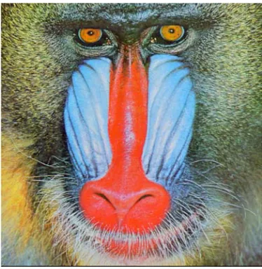
Two images were obtained on which the interpolation algorithms were applied. The first image (Figure 1) is a satellite image of a section of the University of Mines and Technology campus of Ghana. Figure 1 was downloaded using the Google Earth software and is labelled in this study as image A. The second image (Figure 2) is an RGB image of a mandrill, which was downloaded from google webpage. It is labeled as image B in this study.
Figure 1. Satellite Image of a Section of the University of Mines and Technology (Image A).
Figure 2. RGB image of a Mandrill (Image B).
2.2. Image Interpolations
2.2.1. Image Interpolation by Nearest Neighbor Technique
The image interpolation method by the Nearest Neighbor (NN) technique is the most basic and simple method. This method is used to determine the pixel value from the closest pixel to the specified input coordinates, and assigns that value to the output coordinates in [11]. For one-dimension NN interpolation, the numbers of grid points needed to evaluate the interpolation function are two. For two-dimension, NN interpolation, the numbers of grid points needed to evaluate the interpolation function are four. This technique, also known as the point shift algorithm, is given by the Equation (1).
1 1
( ) ( ),
2 2
k k k k
k
x x x x
f x = f x − + < ≤x + − (1)
It can be achieved by convolving the image with a one-pixel width rectangle in the spatial domain. The interpolation kernel for the nearest neighbor algorithm is defined by Equation (2).
1 0 0.5
( )
0 0.5 x h x
x
≤ <
= ≤
(2)
where x is the distance between the point to be interpolated and the grid point being considered.
2.2.2. Image Interpolation by Bilinear Technique
points needed to evaluate the interpolation function is four. Its interpolation kernel is derived from constraints imposed on the general cubic spline interpolation formula. The kernel is composed of piecewise cubic polynomials defined on the unit subintervals (-2, -1), (-1, 0), (0, 1), and (1, 2). Outside the interval (-2, 2), the interpolation kernel is zero. As a result, each interpolated point is a weighted sum of four consecutive input points. This has the desirable symmetry property of retaining two input points on each side of the interpolating region. It gives rise to a symmetric, space-invariant, interpolation kernel in the form of Equation (3).
3 2
30 20 10 00
3 2
31 21 11 01
0 1
( ) 1 2
0 2
a x a x a x a x
h x a x a x a x a x
x
+ + + ≤ <
= + + + ≤ <
≤
(3)
There is again an assumption that the data points are located on the integer grid. The values of the coefficients can be determined by applying the following set of constraints to the interpolation kernel:
i h (0) = 1 and h(x) = 0 for |x| = 1 and 2. ii h must be continuous at |x| = 0, 1, and 2.
iii h must have a continuous first derivative at |x| = 0, 1, and 2.
The first constraint states that when h is centered on an input sample, the interpolation function is independent of neighboring samples. This permits f to actually pass through the input points. In addition, it establishes that the Ck
coefficients in the main interpolation equation are the data samples themselves. This follows that at data point xj as in
Equation (4). 1 0 2 2 ( ) ( ) ( ) k
j k j k
k j
k j k k j
f x C h x x
C h x x − = + = − = − = −
∑
∑
(4)According to the first constraint (Equation 4), h(xj- xk) = 0
unless j = k. Therefore, the right-hand side of Equation (4) reduces to Ck. Since this equals f(xj), it can be seen that all Ck
coefficients must equal the data samples in the four-point interval as given in Equations (5) to (8).
00
1=h(0)=a (5)
1
30 30 30 30
0=h(1 )− =a +a +a +a (6)
31 21 11 01
0=h(1 )+ =a +a +a +a (7)
31 21 11 01
0=h(2 )− =8a +4a +2a +a (8)
Three more equations are obtained from constraint (Equation (3)) i.e. Equations (9) to (11).
' '
10 (0 ) (0 ) a10
a h − h +
− = = = (9)
' 30 20 10 '
31 21 11
3 2 (1 )
(1 ) 3 2
a a a h
h a a a
− +
+ + =
= + + (10)
' '
31 21 11
12a +4a +a =h(2 )− =h(2 )+ =0 (11)
The constraints given in Equations (9) to (11) have resulted in seven equations. However, there are eight unknown coefficients. This requires another constraint in order to obtain a unique solution. By allowing a = a31 to be a
free parameter that may be controlled by the user, the family of solutions given in Equation (12) may be obtained.
3 2
3 2
( 2) ( 3) 1 0 1
( ) 5 8 4 1 2
0 2
a x a x x
h x a x a x a x a x
x
+ ⋅ − + ⋅ + ≤ <
= ⋅ + ⋅ + ⋅ − ≤ <
≤
(12)
Additional knowledge about the shape of the desired result may be imposed upon the Equation (12) to yield bounds on the value of a. The heuristics applied to derive the kernel are motivated from properties of the ideal reconstruction filter, the sinc function. By requiring h to be concave upward at |x| = 1, and concave downward at x = 0 give Equations (13) and (14).
''
(0) 2( 3) 0 3
h = − a+ < → > −a (13)
"(1) 4 a 0 a 0
h = − > → < (14)
2.2.3. Image Interpolation by Bicubic Technique
The characteristics of Image Interpolation by bicubic technique in [12] are as follows:
i Cubic convolution Interpolation determines the pixel value from the weighted average of the 16 closest pixels to the specified input coordinates, and assigns that value to the output coordinates.
ii First, four one-dimension cubic convolutions are performed in one direction and then one more one-dimension cubic convolution is performed in the perpendicular direction.
iii For Bicubic Interpolation, the number of grid points needed to evaluate the interpolation function is 16, two grid points on either side of the point under consideration for both horizontal and vertical directions.
2.2.4. Processing of Image A
Figure 3. Resized Image A: Image A-A.
Figure 3 (Image A-A) was then loaded into the workspace and the interpolation methods (nearest neighbor, bilinear and bicubic) were applied to the image using a scale factor of 5. The codes written for the interpolation methods were run and timed and the results were saved.
2.2.5. Processing of Image B
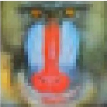
Matlab 2014a was launched and the workspace was connected to the folder which contains Image B (Figure 2). The image was loaded into the workspace and down-sample of the image size using a scale factor of 1/6 was done. The resized or down-sampled image was saved and labelled as Image B-B (Figure 4).
Figure 4. Resized Image B: Image B-B.
Figure 4 (Image B-B) was then loaded into the workspace and the interpolation methods (nearest neighbor, bilinear and bicubic) were applied to the image using a scale factor of 5. The codes written for the interpolation methods were run and timed and the results were saved.
After the enhancement of the images using the interpolation techniques, Images A-A (Figure 3) and B-B (Figure 4) were enhanced using the normal zoom-in feature of windows photo viewer in the computer. This was done in order to show how image enhancement by the interpolation techniques differs from the normal image enhancement or zooming methods of a computer.
3. Results and Discussion
3.1. First Set of Results for Images A-A and B-B
Figures 5 and 6 show images A-A and B-B enhanced using the normal zoom-in feature of the windows photo viewer of a computer.
Figure 5. Enhanced Image A-A using the Normal Zoom-in of Windows Photo Viewer.
Figure 6. Enhanced Image B-B using the Normal Zoom-in of Windows Photo Viewer.
3.1.1. Second Set of Results for Image A-A
Figures 7 to 9 show images A-A enhanced using the three interpolation techniques being treated in this study.
Figure 8. Image A-A Enhanced Using the Bilinear Interpolation Technique.
Figure 9. Image A-A Enhanced Using the Bicubic Interpolation Technique.
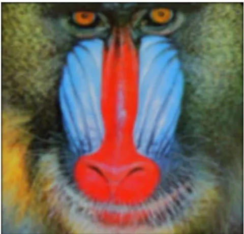
3.1.2. Third Set of Results for Image B-B
The Figures 10 to 12 show images of B-B, enhanced using the three interpolation techniques being used in this study.
Figure 10. Image B-B Enhanced using the Nearest Neighbor Interpolation Technique.
Figure 11. Image B-B Enhanced Using the Bilinear Interpolation Technique.
Figure 12. Image B-B Enhanced Using the Bicubic Interpolation Technique.
3.1.3. Computational Speed of the Three Interpolation Techniques
Table 1 shows the computational speeds for the three interpolation techniques for the enhancement process of the images A-A (Figure 3) and B-B (Figure 4).
Table 1. Computational Speed of the Three Interpolation Techniques.
IMAGES INTERPOLATION TECHNIQUES (COMPUTATIONAL SPEEDS)
NEAREST NEIGHBOR (s) BILINEAR (s) BICUBIC (s)
IMAGE A-A 0.504 0.732 0.912
3.2. Discussion
By visual inspection, It can be seen from the first set of results (Section 3.1.1) that the enhancement using the normal zoom in feature of the windows photo viewer was a failure because both images were very pixelated and the features in the image could not be seen. This shows that the enhancement using the interpolation techniques differs totally from the normal zoom in on the windows photo viewer. The nearest neighbor interpolation generally performed poorly. Both images A-A (Figure 3) and B-B which were enhanced using the nearest neighbor interpolation technique produced a jagged or blocky appearance.
Bilinear Interpolation generated images of smoother appearance than nearest neighbor interpolation, but the
images were however altered in the process, resulting in blurring or loss of image resolution. Evidently, the bicubic interpolation technique produced images better than the other two techniques. The bicubic interpolation technique produced sharp images which eliminated blurring and jagging in the images.
Computational Speed
From Table 1, it could be seen that the fastest among the three techniques used is the nearest neighbor. This is because the nearest neighbor technique had the least computation time followed by bilinear and then bicubic. This can be attributed to the degree of computational complexity of each of the techniques. A generalized table for the comparison of the interpolation techniques based on the results can be found in Table 2.
Table 2. General Comparison of the Three Methods.
INTERPOLATION ALGORITHMS COMPUTATIONAL TIME COMPLEXITY OF ALGORITHM IMAGE QUALITY
Nearest Neighbor low low poor
Bilinear average average average
Bicubic high high good
4. Conclusion
There are a number of interpolation algorithms that could be used to enhance an image. The three most common, nearest neighbor, bilinear and bicubic are compared in this study. Two different images (Multispectral and RGB) were enhanced using the three interpolation techniques. By visual inspection, the bicubic interpolation algorithm gave the best results in terms of image quality, but took the greatest amount of processing time because it needs larger amount of calculations. Considering the computational speeds of the three techniques, the Nearest Neighbour was the fastest among the three having the lowest computational time of 0.504 for image A-A and 0.713 for image B-B. Comparing the complexity of the algorithms, the Nearest Neighbor had the lowest among the three. However, considering the development of modern technology in computers, the bicubic image interpolation technique is adjudged the most suitable amongst the three techniques to be used for image enhancement because it produces sharper images than the other two techniques and has good compromise between processing time and output quality. The results of this particular research can give guidance for a user to choose a suitable interpolation algorithm.
References
[1] Robert G. (2012), “Cubic Convolution Interpolation for Digital Image Processing”, IEEE Transactions on Acoustics, Speech, and Signal Processing, Vol. ASSP-29, Issue 6, pp. 1153-1160.
[2] Thilina S. (2014), “Digital Image Zooming”, www.thilinasameera.wordpress.com. Accessed: March 04, 2018.
[3] Maini, R. and Aggarwal, H. (2010), “A Comprehensive Review of Image Enhancement Techniques”, Journal of Computing, Vol. 2, Issue 3, pp. 8-13.
[4] Huijian, H., Changjin, L. and Jiefei, F. (2012), “The Non-Uniform B-Spline Interpolation Image Enlargement Algorithm”, Journal of Computational and Theoretical Nanoscience, 7 (1), 277-280.
[5] R. G. Keys, Cubic convolution interpolation for digital image processing, IEEE Transactions on Acoustics, Speech, Signal Processing 29 (6) (1981) 1153–1160.
[6] S. D. Bayraker, R. M. Mersereau, A new method for directional image interpolation, IEEE International Conference on Acoustics, Speech, and Signal Processing 4 (1995) 2383–2386. [7] L. Khriji, M. Gabbouj, Directional-vector rational filters for
color image interpolation Proceedings of the Tenth International Conference on Microelectronics (1998), pp. 236–240.
[8] Jiefei, F. and Han Huijian. H. (2010),”Image enlargement based on non-uniform B-spline interpolation algorithm”. Journal of Computer Applications, Vol. 30, Issue 1, pp. 82-84. [9] Bedi, S. and Khandelwal, R. (2013), “Various Image
Enhancement Techniques - A Critical Review”, International Journal of Advanced Research in Computer and Communication Engineering, Vol. 2, pp. 55-67.
[10] Carlson, B. (2012), “Image Interpolation and Filtering”, IEEE Trans on ASSP, Vol. 6, pp. 32-45.
[11] Kassab A. (2012), “Image Enhancement Methods and Implementation in Matlab”, MSc Project, Zapadoceska Univerzita V Plzni, 55pp.
[12] C. Lee, B. Zeng, A novel interpolation scheme for rectangularly subsampled images, International Conference on Image Processing 3 (1999) 787–791.
[14] H. Jiang, C. Moloney, A new direction adaptive scheme for image interpolation, International Conference on Image Processing 3 (2002) 369–372.
[15] A. M. Darwish, M. S. Bedair, S. I. Shaheen, Adaptive resampling algorithm for image zooming, IEE Proceedings-Vision Image and Signal Processing 144 (4) (1997) 207–212. [16] Maeland E. and Gupta S. (2012), “On the Comparison of
Interpolation Methods”, IEEE Transactions on Medical Imaging, Vol. 7, No. 6, pp. 213-217.
[17] Russell, W., S. (1995), “Polynomial interpolation schemes for internal derivative distributions on structured grids,” Applied Numerical Mathematics, Vol. 17, No. 2, pp. 129–171.
[18] Hou, H. and Andrews, H. (1978), “Cubic splines for image interpolation and digital filtering,” IEEE Trans. Acoust. Speech Signal Process, Vol. 26, No. 6, pp. 508–517.
[19] Han, D. (2013), “Comparison of Commonly Used Image Interpolation Methods”, Proceedings of the 2nd International Conference on Computer Science and Electronics Engineering (ICCSEE 2013), pp. 1-4.