R E S E A R C H
Open Access
Simple robust parameter estimation for
the Birnbaum-Saunders distribution
Min Wang
1*, Chanseok Park
2and Xiaoqian Sun
3*Correspondence: [email protected] 1Department of Mathematical Sciences, Michigan Technological University, Houghton, MI, USA Full list of author information is available at the end of the article
Abstract
We study the problem of robust estimation for the two-parameter Birnbaum-Saunders distribution. It is well known that the maximum likelihood estimator (MLE) is efficient when the underlying model is true but at the same time it is quite sensitive to data contamination that is often encountered in practice. In this paper, we propose several estimators which have simple closed forms and are also robust to data contamination. We study the breakdown points and asymptotic properties of the proposed estimators. These estimators are then applied to both simulated and real datasets. Numerical results show that the proposed estimators are attractive alternative to the MLE in that they are quite robust to data contamination and also highly efficient when the underlying model is true.
Keywords: Hodges-Lehmann estimator, Rousseeuw-Croux estimator, Robustness, Breakdown point, Data contamination
Mathematics subject classification: 62F10, 62F12, 62F35
1 Introduction
The two-parameter Birnbaum-Saunders (for short, BS) distribution was originally pro-posed by Birnbaum and Saunders (1969a) as a failure time distribution to describe the total time until the damage caused by the development and growth of a dominant crack grows to a critical level that would cause fracture of failure. The random variableT is said to follow the BS distribution with parametersαandβif its cumulative distribution function (cdf ) is given by
F(t|α,β)=
1
α
t β −
β
t
, 0<t<∞, α, β >0, (1)
where(·)is the cdf of the standard normal distribution, and the parametersαandβare the shape and scale parameters, respectively. This distribution has been widely applied to a variety of quality and reliability engineering problems. For example, Bhattacharyya and Fries (1982) developed fatigue failure models and also discussed the intrinsic rela-tion between the inverse Gaussian distriburela-tion and the BS distriburela-tion. Using the inverse Gaussian approximation to the BS distribution, Park and Padgett (2006) developed var-ious new cumulative damage models and degradation models. Lio and Park (2008) developed a bootstrap control chart based on the BS distribution.
Estimation of the BS parameters is of great interest to researchers and has recently received much attention in the literature. Birnbaum and Saunders (1969b) firstly dis-cussed the MLEs of α and β. Engelhardt et al. (1981) derived the asymptotic joint distribution of the MLEs and showed that the MLEs are asymptotically independent. Achcar (1993) studied the Bayesian estimators based on Jeffreys’ prior and the refer-ence prior and adopted Laplace’s approximations to the posterior marginal distribution of the parameters of interest. Ng et al. (2003) proposed the method-of-moment estimator (MME) of the two parameters. All the above mentioned approaches, except for the MME, have no explicit closed-form solutions, so some numerical approaches are often required to obtain these estimators.
The quality of data is extremely important for parameter estimation and complete data without any contamination is always preferred to achieve a high accuracy on parameter estimation. Unfortunately, in the engineering sciences, there is no guarantee that the col-lected data exactly follow the assumed model. In other words, reliability engineers often face data with deviations from the assumed model especially when studying failure data. Note that the commonly used estimators such as the MLEs are very sensitive to data con-tamination and model departure that are often encountered in many practical situations. Small deviations may induce a large impact on these estimators and a single outlier can even make them break down. This phenomenon motivates many authors to study robust estimation for various distributions; see, for example, Agostinelli et al. (2014), Boudt et al. (2011), Lawson et al. (1997), among others. Of particular note is that many researchers mainly focus on robust estimation for the Weibull distribution and that robust estimation for the BS distribution is quite scant, even though the BS distribution is prevalent in the engineering sciences as an effective model of studying fatigue data.
It deserves mentioning that Dupuis and Mills (1998) developed the robust estimation procedures based on an optimal bias-robust estimator (OBRE) of the BS distribution, whereas the OBRE is not in explicit form and it may suffer from the problem of conver-gence. These observations give rise to the need for some alternative estimators, which should be easy to calculate for practitioners and are also quite robust against a certain amount of data contamination. Recently, Wang et al. (2013) developed a new method for robustly estimating the parameters of the BS distribution, whereas their method is somewhat complicated for practitioners.
The remainder of this paper is organized as follows. In Section 2, we firstly present a summary of the BS distribution and the MLEs, and then provide several alternative esti-mators in explicit closed-form expressions. We also investigate the asymptotic properties of these estimators along with their breakdown points. Section 3 contains an extensive Monte Carlo simulation to compare the behavior of the proposed estimators and that of the MLEs. In Section 4, we illustrate the practical application of all the estimators under consideration through using a real dataset. Finally, some concluding remarks and discussions are given in Section 5.
2 Parameter estimation
If a random variableT follows the BS distribution with the cdf in (1), then T has the probability density function (pdf ) given by
f(t|α, β)= 1 2√2αβ
β
t
1/2 +
β
t
3/2 exp
− 1
2α2
t β +
β
t −2 .
It is well known that this distribution has many attractive properties. (i) The scale parameter β is the median of the distribution, that is, F(β) = (0) = 0.5; (ii) it is positively skewed, with degree of skewness decreasing withα; (iii) for any con-stant κ > 0, it follows that κT ∼ BS(α, κβ); (iv) its reciprocal property (Saunders 1974) holds, that is,T−1 ∼ BS(α, β−1); and (v) if we make the transformationT = β1+2X2+2X(1+X2)1/2, thenXis normally distributed with mean zero and variance
α2/4.
We firstly provide a brief review to the MLEs of the BS distribution. Let T = {t1,t2,· · ·,tn} be a random sample of size n from the BS distribution. The sample
arithmetic and harmonic means are given by
s= 1 n
n
i=1
ti and r=
1 n
n
i=1
ti−1 −1
,
respectively. Leth(·)be the harmonic mean function given by
h(x)=
1 n
n
i=1
(x+ti)−1
−1 .
Then the MLE ofβ, denoted byβˆMLE, can be obtained as the unique positive root of the following equation
β2−β[2r+h(β)]+r[s+h(β)]=0. (2)
OnceβˆMLEis obtained, the MLE ofα, denoted byαˆMLE, is given by
ˆ
αMLE= s ˆ βMLE +
ˆ βMLE
r −2.
Because the uniqueness of the solution for Eq. (2) is guaranteed in the interval(r, s), a one-dimensional root search is adopted in this paper to compute the MLEs instead of their methods; see, for example, Lio and Park (2008).
two estimators ofβ; the other is to develop two estimators ofα. The proposed estimators are explicit closed-form expressions in terms of the sample observations and can thus be easily computed in practical situations. Furthermore, it can be shown that some of them are asymptotically normally distributed and have the highest breakdown point of 50 %.
2.1 The estimators of the parameterβ
Since the parameterβis the median of the BS distribution which satisfiesF(β)=(0)= 0.5, the median is a natural choice as an estimator ofβ. We denote the sample median estimator ofβby
ˆ
βM=median{t
1,t2,· · ·,tn}.
The above median estimator is quite robust and has the highest breakdown point of 50 %. From the asymptotic normality of the median estimator, it can be shown that
√ n
ˆ
βM−β−→D N
0, π(αβ) 2
2 .
Rieck and Nedelman (1991) investigated the relationship between the BS distribution and the sinh-normal distribution and showed that if a random variableT ∼ BS(α, β), thenY =log(T)has the sinh-normal distribution with the cdf and pdf given by
F(y|μ,α)=
2
αsinh
y−μ
2 (3)
and
f(y|μ,α)= 1
α√2π cosh
y−μ 2 exp
− 2
α2sinh
y−μ
2 , (4)
respectively. This distribution has a shape parameterα and a location parameterμ = log(β), which is just the natural logarithm of the scale parameter of the BS distribu-tion. One appealing advantage of using the above relationship is that we transform the asymmetricBS distribution to thesymmetricsinh-normal distribution. It is well known that in the location framework, the Hodges and Lehmann (1963) estimator (for short, HL) of (Hodges and Lehmann 1963) has greater efficiency than does the sample median for symmetric distributions. Thus, it appears to be more beneficial to adopt the HL estima-tor for the parameterμunder the sinh-normal distribution, instead of the sample median of the original BS distribution. The HL estimator is defined as the median ofn(n−1)/2 pairwise averages of observations and can be written as
˜
μ=mediani<j
yi+yj
2
, (5)
which can easily be calculated using thehl.loc(·)function in the package ofICSNPinR language; see R Development Core Team (2011). Also, this estimator has 29 % breakdown point, which means that it remains consistent even if about 29 % percent of the data have been contaminated. In addition, as stated by Rousseeuw and Croux (1993), ‘the Hodges-Lehmann estimator might be viewed as a “smooth” version of the median’. It can be shown that this estimator is asymptotically normally distributed, namely,
√
n(μ˜ − μ)−→D N
0, 1
120∞f(x)2dx
,
Based on the HL estimator in (5), we obtain the back-transformed estimator of the BS parameterβ, denoted byβˆHL, which is simply given by
ˆ
βHL=exp(μ)˜ =exp
mediani<j
yi+yj
2 . (6)
This estimator also has a breakdown point of 29 %. Note that the estimatorβˆHL approx-imately follows the log-normal distribution and that the estimator βˆHL is biased, but consistent forβ.
In what follows, we will adopt the above two estimators ofβto develop the estimator of
αdue to their simplicity and computational ease as well as high breakdown points.
2.2 The estimators for the parameterα
Here, we proposed two robust estimators for the shape parameterα.
Let{t1,t2,· · ·,tn}be a random sample from the BS distribution with the cdf in (1). Note
that−1(0.75)−−1(0.25) = 1.34898 is the distance between the two quartiles of the standard normal distribution, the interquartile range(IQR). The sample IQR is equal to the difference between the third sample quartile (Q3) and the first sample quartile (Q1). To have a normal consistency, we consider the following estimator ofαgiven by
ˆ αIQR
j =
IQR(yj)
1.34898, j=1, 2,
The estimatorαˆjIQR is in simple closed-form with a higher breakdown point of 25 %, indicating that it remains consistent even if about 25 % percent of the data have been con-taminated. Furthermore, by using the Bahadur’s representation theorem (Ghosh 1971), we have
√
nαˆjIQR − α−→D N0, cα2, j=1, 2,
wherecis a constant approximately equal to 2.48/1.3492≈1.363. The quartile estimator ˆ
αIQR
j converges in probability to the parameterα, that is,αˆ
IQR
j p
−→ αforj=1, 2. We observe from Eq. (3) that by lettingY =log(T), we change the estimation problem of theshapeand scale parameters to that of thelocationand scale parameters. We advo-cate the use of (reference) estimator (shortly RC) for the estimator ofα. The RC estimator is given by
ˆ αRC
j =b
|logti−logtj|; i<j
(k),
wherebis a constant factor equal to 1/(√2−1(5/8))≈2.2219 to achieve consistency for standard deviation ofαin the case of the normal distribution above, andk=h2≈n2/4 withh = [n/2]+1 being roughly half the number of observations. The RC estimator is an explicit expression and can be easily calculated using theQn(·)function in the package
3 Monte Carlo simulations
To illustrate the proposed method, we consider Monte Carlo simulation studies with one without contamination and the other involving different kinds of contaminations.
3.1 Numerical results without contamination
We carry out Monte Carlo simulations to compare the performances of the estimators under consideration. We take the sample sizen = 10, 50, 100, and the shape parameter
α=0.5, 1.0, 2.0. Sinceβis the scale parameter, its value was kept fixed atβ =1.0, without loss of any generality.
Inverting the cdf of the BS distributionF(T | α,β) = pgiven by (3), we obtain the following inverse cdf of the form
T =F−1(p)= 1 4
αβ−1(p)+α2β−1(p)2+4β 2
.
Hence, random numbers following the BS distribution can be generated by using a direct inverse method, that is,T =F−1(U)withU∼Uniform(0, 1). Replicate each case 10,000 times. In each simulation, we compute the average biases of each estimator under consideration with its corresponding square root of the mean square error (RMSE) given by
RMSEα=
1
M
M
i=1
ˆ αi−αT
2
and RMSEβ =
1
M
M
i=1
ˆ βi−βT
2 .
The results based onβˆMandβˆHLare presented in Tables 1 and 2, respectively. Several conclusions from the numerical results can be drawn as follows.
(i) The average bias and RMSE of all the estimators significantly decrease asn increases. As expected, for large sample sizes, the performance of the proposed estimators and that of the MLEs are very close in terms of the average bias and RMSE.
(ii) The RC estimatorαˆjRCforj=1, 2outperforms others in terms of the average bias for all the considered cases. Note also that estimation ofαusing the HL estimator
ˆ
βHLis superior than the one using the median estimatorβˆMin terms of the RMSE.
(iii) For the cases without contamination, the estimatorβˆMLEperforms the best as expected. We observe that the performance of the HL estimatorβˆHLis better than that of the median estimatorβˆM. All the estimators ofβbecome closer together as n increases.
3.2 Numerical results with contamination
Table 1Average bias and RMSE (in parentheses) of estimates forαandβ
Estimator ofα Estimator ofβ
n α αˆMLE αˆIQR
1 αˆRC1 βˆMLE βˆM
10 0.5 −0.039 −0.065 −0.000 −0.012 −0.022
(0.117) (0.172) (0.150) (0.156) (0.192)
1.0 −0.087 −0.136 −0.017 −0.040 −0.080
(0.235) (0.343) (0.298) (0.299) (0.412)
2.0 −0.186 −0.273 −0.088 −0.105 −0.331
(0.481) (0.726) (0.597) (0.534) (1.065)
50 0.5 −0.007 −0.015 −0.000 −0.002 −0.003
(0.051) (0.081) (0.059) (0.068) (0.086)
1.0 −0.017 −0.029 −0.003 −0.008 −0.017
(0.101) (0.163) (0.116) (0.128) (0.179)
2.0 −0.035 −0.060 −0.021 −0.018 −0.060
(0.206) (0.334) (0.238) (0.195) (0.379)
100 0.5 −0.004 −0.007 −0.001 −0.001 −0.002
(0.036) (0.058) (0.041) (0.048) (0.063)
1.0 −0.008 −0.014 −0.001 −0.004 −0.007
(0.070) (0.116) (0.080) (0.088) (0.124)
2.0 −0.019 −0.028 −0.011 −0.010 −0.033
(0.144) (0.234) (0.163) (0.135) (0.260)
Model 1 A model with no contamination.
Model 2 A model with5 %of severe contamination; the upper5 %of order statistics are multiplied by 5.
Model 3 A model with5 %of severe contamination; the lower5 %of order statistics are multiplied by1/5.
Table 2Average bias and RMSE (in parentheses) of estimates forαandβ
Estimator ofα Estimator ofβ
n α αˆMLE αˆIQR
2 αˆRC2 βˆMLE βˆHL
10 0.5 −0.039 −0.066 −0.000 −0.012 −0.014
(0.117) (0.171) (0.149) (0.156) (0.164)
1.0 −0.087 −0.141 −0.017 −0.040 −0.048
(0.235) (0.340) (0.297) (0.299) (0.332)
2.0 −0.186 −0.314 −0.078 −0.105 −0.165
(0.481) (0.700) (0.595) (0.534) (0.714)
50 0.5 −0.007 −0.015 −0.000 −0.002 −0.002
(0.051) (0.081) (0.059) (0.068) (0.071)
1.0 −0.017 −0.031 −0.003 −0.008 −0.010
(0.101) (0.162) (0.116) (0.128) (0.139)
2.0 −0.035 −0.071 −0.018 −0.018 −0.029
(0.206) (0.330) (0.238) (0.195) (0.256)
100 0.5 −0.004 −0.004 −0.000 −0.001 −0.001
(0.036) (0.058) (0.041) (0.048) (0.051)
1.0 −0.008 −0.015 −0.001 −0.004 −0.004
(0.070) (0.115) (0.080) (0.088) (0.096)
2.0 −0.019 −0.034 −0.009 −0.010 −0.016
Model 4 A model with5 %of more extreme contamination from a point mass distribution at 50.
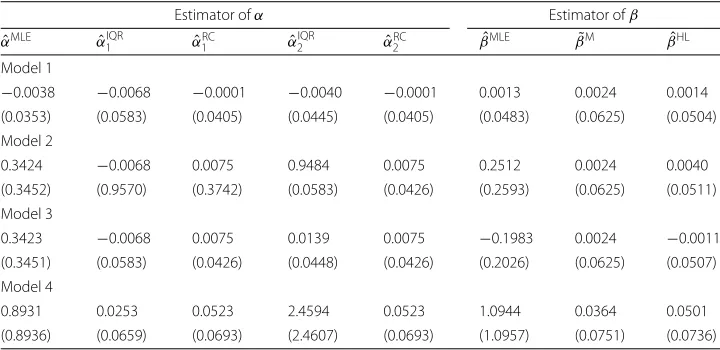
The reference distribution is the BS distribution with the parametersα=0.5 andβ=1. We generate 10,000 samples of sizen = 100 according to the above four scenarios and then calculate the average bias and RMSE of each estimator. The results are shown in Table 3. Some conclusions can be drawn as follows.
(i) For Model 1, that is, there is no contamination, the RC estimatorαˆjRCforj=1, 2 performs the best for estimatingαin terms of the average bias; the MLEβˆis the best one for estimatingβ, but the HL estimatorβˆHLbehaves much similarly. (ii) For Models 2, 3, and 4, that is, contamination presents in the dataset, we observe
that contamination induces a large influence on the average bias and RMSE of the non-robust estimators including the MLEs, especially in the presence of extreme outliers such as the fourth scenario, whereas it has a smaller impact on the proposed estimators.
(iii) For the scale parameter estimation, the HL estimatorβˆHLoutperforms the median estimators in terms of the RMSE, whereas both are quite robust against data contamination.
Which of the two robust estimators, the HL estimator or the median estimator, is prefer-able for the parameterβin the analysis of real lifetime data? Numerical results show that for all the cases considered in this paper, the HL estimatorβˆHLoutperforms the median estimatorβˆM in term of the RMSE. Additionally, the estimator ofαdeveloped based on
ˆ
βHL also slightly outperforms the one usingβˆM in most cases. We thus have a prefer-ence to recommend the HL estimator forβ. It should be mentioned that other simulation results with respect to several other values of the parameterαand different sample sizes have also been conducted, and the conclusions are quite similar and are thus not provided here for brevity.
Table 3Average bias and RMSE (in parentheses) of estimates forαandβwithn=100 under the four models
Estimator ofα Estimator ofβ
ˆ
αMLE αˆIQR
1 αˆ1RC αˆ2IQR αˆRC2 βˆMLE β˜M βˆHL
Model 1
−0.0038 −0.0068 −0.0001 −0.0040 −0.0001 0.0013 0.0024 0.0014
(0.0353) (0.0583) (0.0405) (0.0445) (0.0405) (0.0483) (0.0625) (0.0504)
Model 2
0.3424 −0.0068 0.0075 0.9484 0.0075 0.2512 0.0024 0.0040
(0.3452) (0.9570) (0.3742) (0.0583) (0.0426) (0.2593) (0.0625) (0.0511)
Model 3
0.3423 −0.0068 0.0075 0.0139 0.0075 −0.1983 0.0024 −0.0011
(0.3451) (0.0583) (0.0426) (0.0448) (0.0426) (0.2026) (0.0625) (0.0507)
Model 4
0.8931 0.0253 0.0523 2.4594 0.0523 1.0944 0.0364 0.0501
Table 4Fatigue lifetime data by Birnbaum and Saunders (1969b)
70 90 96 97 99 100 103 104 104 105 107 108 108 108 109 109 112
112 113 114 114 114 116 119 120 120 120 121 121 123 124 124 124 124
124 128 128 129 129 130 130 130 131 131 131 131 131 132 132 132 133
134 134 134 134 134 136 136 137 138 138 138 139 139 141 141 142 142
142 142 142 142 144 144 145 146 148 148 149 151 151 152 155 156 157
157 157 157 158 159 162 163 163 164 166 166 168 170 174 196 212
4 An illustrative example
We illustrate the practical application of the proposed estimators using a real data exam-ple. The dataset from Birnbaum and Saunders (1969b) is the fatigue lifetime of 6061−T6 aluminum coupons cut parallel to the direction of rolling and oscillated at 18 cycles per second. The dataset consists of 101 observations with maximum stress per cycle 31,000 psi and is presented in Table 4.
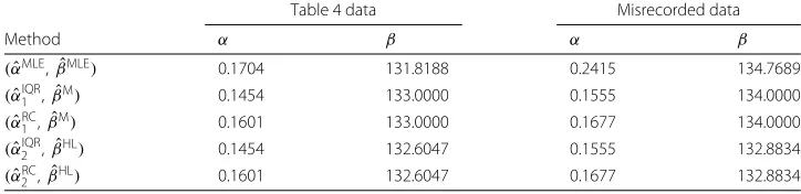
The parameter estimates ofα andβ by all the methods under consideration are pre-sented in Table 5. As mentioned in Section 3, we have a preference over the HL estimator
ˆ
βHLforβ, and thus we just analyze the results based on this estimator for simplicity. It can be seen from Table 5 that in the case of no contamination, most of the proposed esti-mators are in good agreement with the MLEs and that the estiesti-matorsαˆ2RC, βˆHLare slightly different.
To evaluate robustness of the proposed methods, we follow the same scenario by Dupuis and Mills (1998) and assume that the 51st observationt51was misrecorded as 633, instead of 133. It is desirable that the estimated shape and scale parameters should be very similar under the two scenarios, because we already know that the observationt51is a record-ing error. However, it has been observed from Table 5 that the MLEs are heavily distorted by this single outlier and resulted inαˆMLE = 0.2415 andβˆMLE = 134.7689, far from the MLEs witht51 = 133, whereas the proposed robust estimators
ˆ αRC
2 , βˆHL
and
ˆ αIQR
2 , βˆHL
still provided more reasonable results, which are quite close to the estimated values witht51=133.
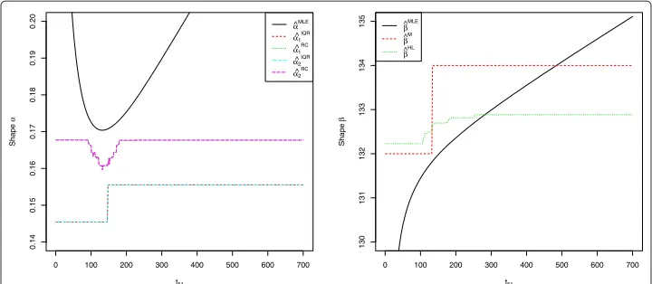
In Fig. 1, we plot the estimated parameters with the same data but where we replace the 51st observationt51by a range of values between 1 and 700. We observe that chang-ing the value oft51 induces a large impact on the behavior of the MLEs, whereas it has little influence on the proposed robust estimators. As expected, the proposed estimators
ˆ αIQR
2 , βˆHL
andαˆ2RC, βˆHLhave some built-in protection against a certain amount of deviation due to data contamination or the measurement errors. In conclusion, the performance of all the proposed estimators is quite satisfactory.
Table 5Comparison between the developed estimators and the MLE through fatigue lifetime data by Birnbaum and Saunders (1969b)
Table 4 data Misrecorded data
Method α β α β
(αˆMLE,βˆMLE) 0.1704 131.8188 0.2415 134.7689
(αˆIQR
1 ,βˆM) 0.1454 133.0000 0.1555 134.0000
(αˆRC
1 ,βˆM) 0.1601 133.0000 0.1677 134.0000
(αˆIQR
2 ,βˆHL) 0.1454 132.6047 0.1555 132.8834
(αˆRC
0 100 200 300 400 500 600 700
0.14
0.15
0.16
0.17
0.18
0.19
0.20
t51
Shape
α
α^MLE
α^1 IQR
α^1 RC
α^2 IQR
α^2 RC
0 100 200 300 400 500 600 700
130
131
132
133
134
135
t51
Shape
β
β ^MLE
β ^M
β ^HL
Fig. 1Estimates for the BS parameters for the fatigue life data in (Birnbaum and Saunders 1969b), where the 51st observation is replaced byt51=1, 2,· · ·, 700
5 Concluding remarks
In this paper, we have developed the two families of the estimators for the BS distribu-tion, which are quite robust to data contamination. Unlike the MLEs, these estimators have simple closed-form expressions with higher breakdown points. For estimation ofβ, we have a preference for the use of the HL estimatorβˆHL, because numerical results show that it remains more accurate than the median estimatorβˆM. Of all the considered esti-mators forαusing the estimatorβˆHL, we recommend the RC estimatorαˆRC
2 , since it has a good trade-off between efficiency and robustness. It deserves to be mentioned that other proposed estimators ofαare also attractive alternatives to the MLE in that they are highly efficient when the underlying model is true.
In summary, we have a preference for the RC and HL estimatorsαˆRC2 , βˆHLfor esti-mating(α, β), because it has been shown to be simple, very effective, and quite robust against model departure that often occurs in many practical situations. Note that cen-sored data occur commonly in the field data from reliability tests, so a possible extension of the proposed estimators for the censored data will be investigated in the future.
Competing interests
The authors declare that they have no competing interests.
Authors’ contributions
MW initiated and carried out the study. MW drafted the manuscript. XS and CP participated in the discussion and proofread the manuscript. All authors read and approved the final manuscript.
Acknowledgements
The authors thank the Editor Carl Lee and the two anonymous reviewers for their comments which have improved the appearance of this paper.
Author details
1Department of Mathematical Sciences, Michigan Technological University, Houghton, MI, USA.2Department of Industrial Engineering, Pusan National University, Geumjeong-gu, Busan, Republic of Korea.3Department of Mathematical Sciences, Clemson University, Clemson, SC, USA.
Received: 3 September 2015 Accepted: 16 November 2015
References
Achcar, JA: Inferences for the Birnbaum-Saunders fatigue life model using Bayesian methods. Comput. Statist. Data Anal. 15, 367–380 (1993)
Bhattacharyya, G, Fries, A: Fatigue failure models−birnbaum-saunders vs. inverse Gaussian. Reliability IEEE Trans. 31, 439–441 (1982)
Bickel, PJ, Lehmann, EL: Descriptive statistics for non-parametric models III: Dispersion. Ann. Statist.4, 1139–1158 (1976) Birnbaum, ZW, Saunders, SC: A new family of life distributions. J. Appl. Probability.6, 319–327 (1969a)
Birnbaum, ZW, Saunders, SC: Estimation for a family of life distributions with applications to fatigue. J. Appl. Probability. 6, 328–347 (1969b)
Boudt, K, Caliskan, D, Croux, C: Robust explicit estimators of Weibull parameters. Metrika.73, 187–209 (2011) Dupuis, D, Mills, J: Robust estimation of the Birnbaum-Saunders distribution. IEEE Trans. Reliab.47, 88–95 (1998) Engelhardt, M, Bain, LJ, Wright, FT: Inferences on the parameters of the Birnbaum-Saunders fatigue life distribution based
on maximum likelihood estimation. Technometrics.23, 251–256 (1981)
Ghosh, JK: A new proof of the Bahadur representation of quantiles and an application. Ann. Math. Statist.42, 1957–1961 (1971)
Hodges, JL Jr, Lehmann, EL: Estimates of location based on rank tests. Ann. Math. Statist.34, 598–611 (1963) Lawson, C, Keats, J, Montgomery, D: Comparison of robust and least-squares regression in computer-generated
probability plots. Reliability IEEE Trans.46, 108–115 (1997)
Lio, YL, Park, C: A bootstrap control chart for Birnbaum-Saunders percentiles. Qual. Reliability Eng Int.24, 585–600 (2008) Ng, HKT, Kundu D, Balakrishnan, N: Modified moment estimation for the two-parameter Birnbaum-Saunders distribution.
Comput. Statist. Data Anal.43, 283–298 (2003)
Park, C, Padgett, W: Stochastic degradation models with several accelerating variables. Reliability, IEEE Trans.55, 379–390 (2006)
R Development Core Team, R: A Language and Environment for Statistical Computing. R Foundation for Statistical Computing, Vienna, Austria (2011). ISBN 3-900051-07-0
Rieck, JR, Nedelman, JR: A log-linear model for the Birnbaum-Saunders distribution. Technometrics.33, 51–60 (1991) Rousseeuw, PJ, Croux, C: Alternatives to the median absolute deviation. J. Amer. Statist. Assoc.88, 1273–1283 (1993) Saunders, SC: A family of random variables closed under reciprocation. J. Amer. Statist. Assoc.69, 533–539 (1974) Shamos, MI: Geometry and statistics: problems at the interface. In Algorithms and complexity (Proc. Sympos.,
Carnegie-Mellon Univ., Pittsburgh, Pa., 1976). Academic Press, New York (1976)
Wang, M, Zhao, J, Sun, X, Park, C: Robust explicit estimation of the two-parameter Birnbaum-Saunders distribution. J Appl. Stat.40, 2259–2274 (2013)
Submit your manuscript to a
journal and benefi t from:
7 Convenient online submission
7 Rigorous peer review
7 Immediate publication on acceptance
7 Open access: articles freely available online
7 High visibility within the fi eld
7 Retaining the copyright to your article