Automatic Diagnosis of Performance Problems in Database Management Systems

(1)

Automatic Diagnosis of

Performance Problems in

Database Management Systems

by

Darcy G. Benoit

A thesis submitted to the School of Computing

in conformity with the requirements for the degree of Doctor of Philosophy

Queen's University

Kingston, Ontario, Canada

June 2003

(2)

Abstract

Database performance is directly linked to the allocation of the resources used by the Database Management System (DBMS). The complex relationships between numerous DBMS resources make problem diagnosis and performance tuning complex and time-consuming tasks. Costly Database Administrators (DBAs) are currently needed to initially tune a DBMS for performance and then to retune the DBMS as the database grows and workloads change. Automatic diagnosis and resource management removes the need for DBAs, greatly reducing the cost of ownership for the DBMS. An automated system also allows the DBMS to respond more quickly to changes in the workload as performance can be monitored 24 hours a day. An automated diagnosis and resource management system allows the DBMS to improve performance for both static and dynamic workloads.

One of the key issues in automatic resource management is the capability of the system to diagnose resource problems. Diagnosis of the resource allocation problem is the first step in the process of tuning the resources. In this dissertation, we propose an automatic diagnosis framework and algorithm that can be used to diagnose DBMS resource problems. We formally define the DBMS diagnosis problem and analyze problem complexity. We develop a model to diagnosis the DBMS and demonstrate the ability of the model to correctly identify system bottlenecks for a generic OLTP workload. We

(3)

modify the OTLP workload to further demonstrate the ability of the diagnosis system to handle changing workloads.

The diagnosis system is evaluated by comparing the performance of the DBMS workload tuned by the diagnosis system to the performance of the same workload tuned by an expert and by the Performance Tuning Wizard software included with our test database. Achieving workload performance that is close to or better than these tuning methods will deem the diagnosis system a success.

The contributions of this dissertation include the forma lization of the diagnosis problem, an analysis of the complexity of the problem, the development and implementation of models to demonstrate that the diagnosis process can be successfully automated and the presentation of a generic diagnosis system that can be adapted to other software systems that rely on resource feedback for performance tuning.

(4)

Acknowledgements

My journey through university has been a long a winding road which has taken me across the paths of many interesting and helpful people, of which there are too many to mention. It is due to these people that my journey has been worthwhile, for the knowledge that I have received from books has paled in comparison to all that I have learned from those close to me. It is with this in mind that I wo uld like to thank those who have helped me though this process.

First and foremost, I would like to thank my supervisor Patrick Martin, who has been extremely supportive and patient in dealing with me. My journey has not always been easy, but he has been with me every step of the way – prodding when I needed prodding, dispensing advice when needed, and generally guiding me along my path. I hope that he is pleased with the final results.

I would also like to thank Wendy Powley, who has helped me solve many problems during the course of my stay at Queen’s. Without her help my journey would have been significantly more difficult. She deserves more praise that I will ever be able to bestow upon her.

Along a research vein, I would like to thank IBM Canada and the IBM Center for Advanced Studies for their support on this project.

(5)

To everyone else in the School of Computing at Queen’s, I would like to express my gratitude. Irene, Debby, Lynda and Sandra have all gone beyond the call of duty to help me when needed, as have Tom, Gary, Dave and Richard when I was having computer troubles. To the softball team and those involved in lively debates in the coffee room – you are in some of my best memories of Queen’s.

Last, but not least, I would like to thank my family and my wife, Elizabeth. Their love, support and sometimes gentle prodding were key in helping me complete my journey. It is their faith in me that made my journey worthwhile.

(6)

List of Figures

Figure 1 - Example decision tree. ... 16

Figure 2 – Overview of the Diagnosis Models... 33

Figure 3 - The Quartermaster Architecture. ... 34

Figure 4 - ER diagram of the formal resource definition... 37

Figure 5 - ER diagram of the resource model... 40

Figure 6 - An example resource model. ... 40

Figure 7 - An example of a generated forward resource tree... 43

Figure 8 - An example of a generated reverse resource tree. ... 44

Figure 9 - ER diagram for the workload model... 46

Figure 10 - Sample Diagnosis Tree. ... 49

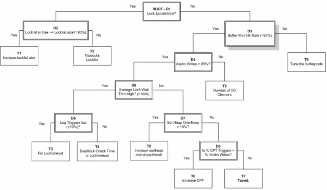
Figure 11 - The initial diagnosis tree... 52

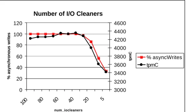
Figure 12 - The impact of I/O cleaners on performance. ... 58

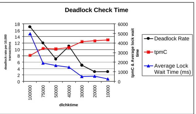
Figure 13 – The impact of deadlock check time on performance. ... 61

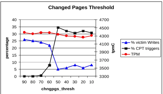
Figure 14 - The impact of the changed pages threshold resource on performance. ... 62

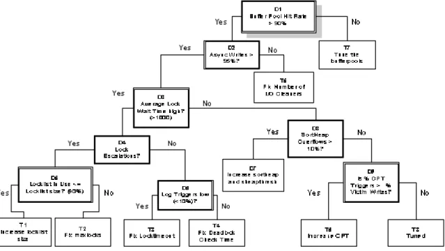
Figure 15 - The tuned diagnosis tree. ... 64

Figure 16 - The effects of the Log Buffer Size on performance... 66

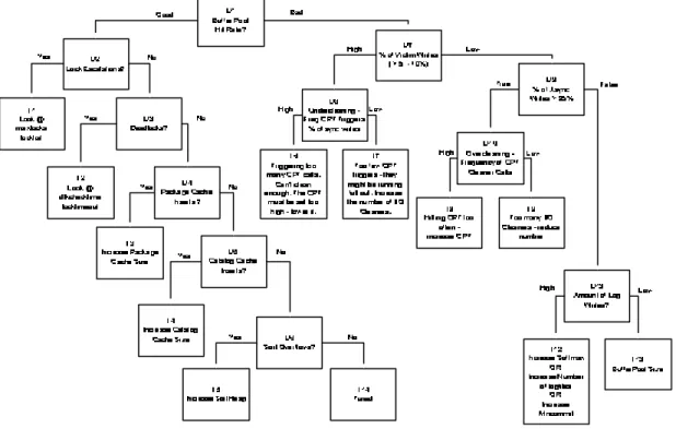
Figure 17 - Proposed generic diagnosis tree. ... 67

Figure 18 - Evaluation Process... 73

Figure 19- Throughput results for the original workload on a small database... 84

Figure 20 - Reverse resource tree with Locklist Size as root... 87

Figure 21 - Reverse resource tree with I/O Cleaners as root... 88

Figure 22 - Throughput results for the diagnosis of the original workload on a large database... 90

Figure 23 - Throughput results for the diagnosis of the modified workload on a small database... 93

(10)

Figure 25 - The effect of sort overflows on sort query response time... 97

Figure 26 - Throughput results for the changed workload on a small database. ... 99

Figure 27 - Throughput results for the changed wo rkload on a large database. ...101

Figure 28 - TPC-C table schema. ...121

Figure 29 - Confidence interval equation...131

Figure 30 - Forward resource tree for the number of I/O cleaners resource. ...140

Figure 31 - Reverse resource tree for the number of I/O cleaners resource...141

Figure 32 - Forward resource tree for the deadlock check time resource. ...141

Figure 33 - Reverse resource tree for the deadlock check time resource...141

Figure 34 - Forward resource tree for the lock timeout resource. ...142

Figure 35 - Reverse resource tree for the lock timeout resource. ...142

Figure 36 - Forward resource tree for the locklist size resource. ...142

Figure 37 - Reverse resource tree for the locklist size resource. ...143

Figure 38 - Forward resource tree for the sort heap size resource. ...143

Figure 39 - Reverse resource tree for the sort heap size resource. ...143

Figure 40 - Forward resource tree for the sort heap threshold resource...144

(11)

List of Tables

Table 1 – Example resources for diagnosis tree tuning. ... 55

Table 2 - Statistical analysis of test workload. ... 71

Table 3 - DBMS resource values... 75

Table 4 – Tuning strategy... 76

Table 5 - DBMS tuning scenarios... 77

Table 6 – Transaction frequencies for the original and modified workloads... 78

Table 7 - Diagnosis of the original workload on a small database... 80

Table 8 - Diagnosis of the original workload on a large database. ... 90

Table 9 - Diagnosis of the modified workload on a small database. ... 92

Table 10 - Diagnosis of the modified workload on a large database... 94

Table 11 - Diagnosis of the changed workload on a small database. ... 98

Table 12 - Diagnosis of the changed workload on a large database. ...100

Table 13 - TPC-C data relations...121

Table 14 - Transaction requirements...122

(12)

Chapter 1

Introduction

A DataBase Management System (DBMS) is an application that allows a user to create, access, and maintain a collection of related data. A DBMS is a complex system that is composed of a collection of subsystems, each with a specific task. It is the job of the DBMS software to control each of these smaller subsystems during the life of a database. Due to the inherent competition for system resources, it is understandable that achieving a high level of performance from a DBMS is a difficult task. System resources are allocated for use by the DBMS through DBMS resource settings. The initial difficulty confronted whe n tuning a DBMS is determining which of the numerous resources need to be adjusted in order to solve the performance problem. In this dissertation, we consider the difficulties associated with diagnosing DBMS performance problems and propose a method for automating the diagnosis process.

(13)

1.1 Definitions

In order to discuss the various issues involved with DBMS performance, several concepts must first be introduced.

Resource – A resource is a piece of software or hardware that is in limited supply. An example of a hardware resource is the physical memory in the system. An example of a software resource is a logical limit placed on the number of allowed concurrent processes.

Resource Tuning – Resource tuning is the process of determining how to adjust the setting for a particular resource in order to alleviate a bottleneck in the DBMS. Determining how to adjust a resource involves knowledge of how that particular resource affects the running system as well as how adjusting that resource affects other resources.

DBMS Tuning – DBMS tuning is the process of increasing or decreasing the performance of the DBMS by altering the amount of physical and logical resources available to the DBMS.

Diagnosis – DBMS diagnosis is the process of determining which of the database resources needs to be adjusted in order to solve a performance problem. Once the offending resource has been identified, we perform resource tuning to determine how to adjust the problem resource.

(14)

1.2 Motivation

A DBMS has the responsibility for accessing and maintaining large amounts of data. Maintaining data integrity and supporting concurrent users introduces a significant amount of overhead to a DBMS. This overhead decreases the ability of the DBMS to serve the data to the users quickly. We must decrease overhead while maintaining data integrity and providing information to the users as quickly as possible.

DBMS performance is regulated by adjusting DBMS resource parameters. The large number of tuning parameters and the complexity of workloads makes achieving and maintaining peak DBMS performance a non-trivial task [SHI00] [CHA00] [WEI94]. DataBase Administrators (DBAs), who are the people with the knowledge and expertise needed to tune DBMSs, are scarce and expensive to employ [CHA99] [LOM99] [WEI94].

The process of DBMS tuning can be broken down into two distinct tasks: diagnosis and resource adjustment. Diagnosis involves determining which of the resources in the DBMS is responsible for the performance problem. Resource adjustment involves altering the settings for a particular resource (and others that may be related to it) in order to achieve better performance. Resource adjustment is also referred to as “resource tuning”. As databases increase in size and complexity, the ability to manually control performance becomes “impractical” [BRO94] [BRO95]. Several calls for the automation of the diagnosis and tuning processes ha ve been made in recent years [BER98] [BRO94]

(15)

[CHA00] [CHA99] [LOM99] [MAR00] [WEI94]. Automation would allow the DBMS to quickly achieve peak performance without any human interaction.

It is important to clarify that two different levels of “tuning” exist for DBMSs. In one case, DBMS resources are adjusted in order to increase or maintain performance. In the other case, performance tuning consists of application optimization, data placement concerns, hardware issues and other factors external to the DBMS. This dissertation will focus on the adjustment of DBMS resources as the method of affecting performance.

DBMS tuning involves the collection and analysis of DBMS performance statistics in order to determine the cause of the performance problem [IBM00]. The statistics collected may be simple to read and understand, or they may need to be calculated from other data and then analyzed. It is a time-consuming task for a DBA to analyze the large amount of performance data that can be collected from a running DBMS. A DBA must narrow down the amount of data to be analyzed by considering the type of performance problem and then rule out some of the resources.

By automating the analysis of the performance data, it is possible to consider a large amount of data in a very short period of time. Automatic diagnosis should lead to a more thorough inspection of all of the data while quickly producing a list of possible culprit resource allocations.

(16)

The inevitable increase in hardware performance will ultimately lead to more powerful computers embedded in various systems and Internet appliances. Appliances that store and manage information will be candidates for embedded DBMSs. The interfaces associated with such Internet appliances will not likely provide the option for adjusting DBMS parameters, so the underlying DBMS in such a device will have to be self-managing [BER98].

A DBMS is a natural choice as an interface to provide large amounts of data on the Internet. Unfortunately, the Internet does not provide a stable workload for a DBMS. The workload changes as the number of people browsing increases and decreases throughout the day. It is impossible for a DBA to tune a database quickly enough to keep up with a consistently shifting workload. Automating the diagnosis and tuning processes will enable the DBMS to dynamically manage the available resources in these situations.

Cost is another consideration in the quest for a self- managing DBMS. DBAs are expensive to hire, even for short durations. A full-time DBA is a heavy burden for small and medium- sized businesses. Automation of the tuning process can remove much of the need for a DBA. It can also mean less hardware cost since the DBMS can make the best use of available resources. At present, many companies use overpowered machines to run their DBMSs in order to compensate for inadequate performance tuning. An overpowered machine is able to support mediocre performance tuning while handling shifting workloads with the extra hardware resources. Automatic tuning provides better usage of the hardware resource, thereby eliminating the need to buy an overpowered machine.

(17)

1.3 Contributions

An algorithm is proposed to automatically diagnose DBMS performance problems. The algorithm uses a diagnosis tree and a resource model along with hardware and workload models to diagnose resource bottlenecks. The diagnosis algorithm is constructed as part of the Quartermaster framework, which is a goal-oriented framework for diagnosing and tuning DBMS resources [BEN99]. Such a diagnosis and tuning framework can be applied to other types of software systems where performance is an issue.

The contributions of this dissertation are the following:

• a formal description of the DBMS diagnosis problem;

• an analysis of the complexity of the diagnosis problem;

• the development and implementation of models to demonstrate successful automation;

• the development of a generic diagnosis system that can be adapted to other software systems

• a systematic experimental evaluation of our approach as compared to an experienced DBA and the DB2 Tuning Wizard

This dissertation shows that the collection of underlying performance data can be used to diagnose performance problems, allowing an automated system to manage and control the resources.

(18)

1.4 Evaluation

The diagnosis model was implemented and tested using IBM’s DB2/UDB. The throughput resulting from each complete diagnosis was compared to various throughput values obtained by using the DB2 Tuning Wizard, a performance application included with the DBMS. Although DB2 was used as an example throughout, the principles used in the creation of the diagnosis system can be applied to other DBMSs as the workloads are not inherently linked to the DB2 software.

1.5 Organization of Thesis

Chapter 2 of this dissertation describes approaches to DBMS diagnosis proposed in the literature. Chapter 3 describes the models used for DBMS diagnosis and explains how the models work together to diagnose a DBMS. Chapter 4 explains the process used to create and tune the diagnosis tree. Chapter 5 presents the results returned from testing our system on a working DBMS. Results are discussed along with the effectiveness of the diagnosis algorithm. Chapter 6 concludes the dissertation by summarizing the results of the research and presenting additional areas of research in the area of automatic diagnosis.

(19)

Chapter 2

Related Work

Related literature has provided information in two distinct areas: previous work on automating DBMS tuning and approaches to the general problem of diagnosing faults in systems. The chapter is divided into four sections. The first section reviews DBMS tuning literature, focusing on the issues of general resource management as well as tuning algorithms for specific resources. The second section introduces the area of diagnosis and presents three different approaches to diagnosing faults in generic systems. The third section discusses how the related work can apply to our proposed system. The final section presents DBMS benchmarks, invaluable tools for evaluation and tuning.

2.1 Previous Efforts

Several efforts have been made in the area of automating the control of DBMS resources. Automating resource management requires that the automated system be able both to diagnose the resource causing the performance problem as well as to properly adjust the

(20)

resource to remove the bottleneck. Each previous effort falls either into the category of automated diagnosis or automated tuning.

2.1.1 Automated Diagnosis

Automated DBMS resource management is the ultimate goal for work in the area of resource management. The following papers address the issue of automating the diagnosis process.

Chaudhuri and Weikum present the idea that the current method of controlling resources in DBMSs is outdated and that a new database system architecture must be considered [CHA00]. They argue that the present model has an overloaded feature set, a query language that is difficult to use, unpredictable performance, overly difficult tuning and various other problems. They believe that the best way to solve the problems facing DBMSs today is by recreating the database management system with a RISC-style architecture. They believe that the performance tuning problems will be solved by restructuring DBMSs into better defined components that are easier to tune. By reducing the number of components involved in the tuning process, automatic resource tuning for DBMSs will be achievable.

Hellerstein has proposed an architecture for a generic automated tuning system (ATS) that uses “a feedback control loop that is layered on top of a target system” [HEL97]. This approach recognizes the complexity associated with performance tuning for all types of computer systems. Other work by Hellerstein and others assesses the application of

(21)

“control theory to the evaluation of controllers” used for software management [PAR01]. Hellerstein also points out the desirability of having a proactive resource management system that can detect problems before they occur as opposed to a reactive system that merely fixes the performance of a degraded system.

Hart et al propose a method to isolate performance problems of systems where performance data is stored in multidimensional databases (MDDBs) [HAR99]. This system is designed to use performance data stored in an MDDB to determine the source of the performance problem. The proposed diagnosis system is applicable to any computer system where performance data is stored in an MDDB. The diagnosis system does not address the problem of adjusting the resources once a problem has been diagnosed.

Bigus et al have recently proposed a generic agent for automated performance tuning [BIG00]. The generic agent is designed to support tuning for systems where no prior knowledge is known to systems where effective resource controllers exist. The generic agent used in the automatic tuning process relies heavily on intelligent control. The test system presented in the paper depends on a neural prediction agent that learns the system model, a neural prediction agent that is adapted to determine the appropriate control settings and an agent responsible for monitoring the workload and performance. The test system is a Lotus Notes server. The automated resource management system is able to reduce the queue length in the server over time.

(22)

Weikum et al address the need for automatic memory management in data servers [WEI99]. The paper surveys the possible approaches to memory management such as the self-tuning of cache memory and exploiting distributed memory and speculative prefetching for data and web servers.

2.1.2 Automated Tuning

Resource management can only be completely automated if system resources can be automatically adjusted to increase system performance. Many papers and approaches exist in the area of resource tuning. This section overviews the various approaches to this problem.

Several papers exist in the area of automatic memory tuning for DBMSs. Brown et al

explore the area of automatic memory management [BRO93] [BRO94] [BRO95]. The main focus of the research work presented in these papers is the relationship between the user-defined goals associated with classes of transactions and the allocation of memory resources in the buffer pool. Brown also considers adjusting multiprogramming levels instead of memory to achieve the same result [BRO94]. Brown’s work approaches the idea of tuning as a goal-oriented problem where the “optimal” resource allocation is when all of the workload goals are achieved.

Chung et al are also interested in goal-oriented buffer pool management [CHU95]. The approach by Chung [CHU95] differs from Brown’s [BRO95] in that the performance index is not calculated based on the I/O response times for transaction classes but by

(23)

measuring the response time of the buffer pool. Buffer pool performance indexes are calculated and they attempt to achieve a “lexicographically minimal performance index vector” by adjusting the size of the buffer pools [CHU95].

Martin et al present a “dynamic reconfiguration algorithm” to resize automatically buffer pools based on class goals set by an administrator [MAR00]. The reconfiguration algorithm takes into consideration the goals set for each of the transaction classes in the workload and uses response times as a basis for reallocating buffer pool memory. An “Achievement Index” is used to determine if a transaction class meets its goals by comparing actual response times with goal response times. Cost estimate equations are used to estimate the effect of moving memory from one buffer pool to another. Buffer pool memory is reallocated until all response times fall within a specified percentage of the required goals.

Xu et al approach the problem of automated memory management by addressing the issue of buffer pool configurations [XU02]. One key memory management issue is the assignment of tables and indexes to particular buffer pools. Assigning two fundamentally different tables to the same buffer pool may result in contention for memory and adversely affect performance. The approach taken involves defining a feature vector for each database object and then using a data-clustering algorithm to define similar groups of database objects. The resulting groups are then assigned to buffer pools that are sized appropriately, resulting in a configuration that performs as well as one designed by an expert DBA.

(24)

Chaudhuri and Narasayya approach the area of dynamic resource allocation from the perspective of automating statistics management for the DBMS query optimizers [CHA00-2]. DBMSs use statistics about the data stored in the database to determine the query plan used. Knowing which statistical information is needed is currently left to the DBA. This paper presents techniques for automatically determining which statistics are essential and which statistics are non-essential.

Agrawal et al investigate automating the selectio n of indexes and materialized views for DBMSs [AGR00]. Both indexes and materialized views can greatly increase DBMS performance if the correct set exist during query execution. Maintaining every possible index or materialized view is not possible, resulting in an incomplete set in the DBMS. Choosing the indexes or materialized views that will best serve the workload is a difficult decision. Agrawal et al present algorithms and an architecture that can identify a small set of candidate materialized views and indexes.

Weikum et al explore the subject of automated tuning systems for DBMSs with the “Comfort Automatic Tuning Project” [WEI94]. The project exp lores system design principles needed to create an automated tuning system for DBMSs. The paper reiterates the need for dynamically adjustable resource parameters to allow the feedback loop to adjust resources while the workload is running. Several tuning algorithms for specific problems such as load control for locking and self-tuning memory management are described.

(25)

2.2 Diagnosis

“Diagnostic reasoning requires a means of assigning credit or blame to parts of the model based on observed behavioral discrepancies” [deK92]. Using this definition of diagnostic reasoning, we should be able to use diagnostic reasoning to determine what resources are affecting the performance of a DBMS. We consider two different types of diagnostic systems – rule-based diagnosis and model-based diagnosis.

Rule-based diagnosis

Building a traditional rule-based diagnosis system for troubleshooting first involves the accumulation of data from experts [DAV92] [PAU98] [RYM92]. Empirical associations and rules about objects are created by the experts most familiar with the system at hand. This information is then used to build a rule-based diagnosis system to troubleshoot the system. Such rule-based diagnosis systems are very dependent on the device for whic h they are designed and require a new set of rules for each new device or version of the device. Gathering information from experts can also be a difficult task, as a large body of information and experience may be needed before a useful algorithm can be devised [DAV92]. An example of a rule-based system is XCON, an expert system used to configure DEC computers. Approximately 500 rules were needed to configure the VAX 780 computer. The number of rules increased to 6000 as additional models were added to the rule base [LUG93]. Gathering and programming rules of this type is a time-consuming and difficult task.

(26)

A variation on rule-based diagnosis involves the use of decision trees [DAV92] [RYM92]. Decision trees stem from the state space representation of some problems [LUG93]. In a state space representation of a problem, states of the solved problem are stored at each node in the tree. The tree is then traversed, using the rules stored at the nodes along with facts about the current world state to solve the problem. The tree traversal can be either goal-directed, where the goal is known and the tree is traversed to find the data, or data-directed, where the data is known and we traverse the tree to determine the goal [LUG93].

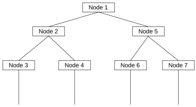
In a decision tree, rules are stored at each node. As the tree is traversed, each node is evaluated and the result determines which branch of the tree will be followed. As nodes in the tree are evaluated and branches of the tree are traversed, other branches and nodes in the tree are excluded or “pruned” during the traversal [LUG93]. Pruning the tree can quickly reduce the number of possible solutions while focusing on those solutions most likely to solve the problem. For example, consider the decision tree in Figure 1. If the decision made at Node 1 causes Node 5 to be next to be traversed, then in that single step the entire left side of the tree under Node 2 is pruned from the search space.

(27)

Figure 1 - Example decision tree.

Model-based Diagnosis

In diagnostic reasoning, a model of the system is used to determine what parts of the system are not performing correctly. The model of the system is presumed to be correct and any differences between the model and the actual system are used to point out malfunctions in the system. Model-based diagnosis is acknowledged as a wide ranging area [deK92]. Model-based diagnosis includes troubleshooting mechanical devices, circuits, and modeling physical or biological systems [deK92].

The primary application area for diagnostic reasoning is electronics, specifically circuits and other multi-component systems [deK89], [deK92], [MOZ91]. The key issue with systems of this nature is to find the component or components that are causing the

Node 1

Node 4

Node 3

Node 6

Node 7

Node 5

Node 2

(28)

problem and to replace or repair them. This requires the component to be performing incorrectly, as diagnosis in a circuit is really a test of correctness. Problems in circuits can usually be traced to the malfunction of a component – such as an adder that is not adding or a broken XOR switch. Component error can be quantified and isolated, making it identifiable to the diagnostic process. This is not the case when diagnosing a DBMS. In DBMSs, resources do not have a quantifiable “broken” state; instead, they do not perform to capacity. We do not know the upper performance limit of many resources as the capacity of the resource is unknown and is dependent on many factors. Since there is no “broken” part in the DBMS, the traditional methods of testing for malfunctioning components do not apply.

When diagnosing circuits and other component-based systems, the solution to the problem usually involves the replacement of the broken component. After replacing the broken component the circuit is retested to ensure that replacement part is functioning properly. Alleviating a bottleneck in a DBMS system involves the reallocation of resources. There is no “correct” allocation for any one particular resource in a DBMS. What may be an optimal allocation for one workload and computer system may not work for a different workload or computer system.

A model of the DBMS system is needed to use model-based diagnostic reasoning for system diagnosis. Davis and Hamscher [DAV92] discuss the issue of systems that are either too simple or too complex to model. The complex end of the spectrum is bound by problems “involving subtle and complicated interactions in the device, interactions whose

(29)

outcome is too hard to predict…” [DAV92]. The relationships between resources in a DBMS are complex and not well understood. Resources can be related either by the sharing of an underlying physical resource, or by having a software dependence on another resource in the system. The complex web of relationships between physical and logical resource allocations results in the relationship between resources being unclear. This already complex model is further complicated by the workload the DBMS is expected to run. Accurately modeling the DBMS is not presently possible due to the complexities of the system.

2.2.1 Optimization

“Optimization is a technology for calculating the best possible utilization of resources needed to achieve a desired result” [EOP02]. Determining the best utilization of resources depends on the boundaries set by those trying to solve a given problem. In one case, the best utilization of resources may mean solving the problem in the least amount of time. Another case may require that the problem be solved with the least amount of resources. A third case may involve maximizing the throughput for the given problem. In all of these cases, optimization involves maximizing or minimizing one aspect of the problem such as time, throughput or resources. With respect to the DBMS resource problem, we could apply optimization techniques to maximize the throughput of the system or to minimize the amount of resources used by the system. Either method would produce the desired effect of better performance with fewer resources. Several different optimization algorithms are reviewed in here – generic optimization, dynamic programming and linear programming. Some of these optimization algorithms are very

(30)

specific to a particular problem, while others are more generic and can be applied to several different types of problems [MOL89].

Generic Optimization

Optimization usually involves finding a maximum or minimum value for the presented problem by solving a series of equations that are used to model the system [GAS75]. We must therefore first be able to create a series of equations to model the system. This is possible only if the relationships between the various resources are documented and well defined.

In the case of a DBMS system, there are simply too many resources (typically hundreds) to consider defining every interdependency between all of the resources. The complexity of creating a series of equations for a generic optimization algorithm to use far outweighs the cost associated with diagnosing the DBMS.

Dynamic Programming Model

Dynamic programming is a technique for solving many different types of optimization problems [CUR97]. Dynamic programming was introduced by Richard Bellman in 1957 [BEL57]. He introduced the idea of the Principle of Optimality that states:

“An optimal policy has the property that whatever the initial state and initial decision are, the remaining decisions must constitute an optimal policy with regard to the state resulting from the first decision”

(31)

Bird and de Moor [BIR93] state that dynamic programming can be used to solve an optimization problem if the solution to that problem is composed of optimal solutions to subproblems. This requires that the initial problem be divided into smaller subproblems that have optimal solutions. In general, dynamic programming is used where a sequence of decisions is needed to solve a particular problem. By computing various solutions to smaller subproblems, dynamic programming reuses the solutions to various subproblems as a way of avoiding unnecessary computation [CUR96].

We are not able to divide the initial DBMS diagnosis problem into smaller, solvable optimization problems because of the level of interaction between the various DBMS resources. It is not possible to find the optimal allocation for one resource without taking into consideration the allocations of other resources. Without the ability to break the larger problem into smaller, solvable subproblems, the dynamic programming solution is impractical.

Linear Programming Model

Linear programming problems are a subset of general ma thematical problems in which the description of the mathematical model of the problem can be stated using linear equations [GAS75]. Linear equations are those equations which, when plotted on a graph, are straight lines. Linear programming was developed and introduced by American George B. Dantzig in 1947 as a method for solving linear problems presented by the U.S. Air Force. Once introduced to the world, it became clear that linear programming could be used for a wide range of production and optimization problems. The original simplex

(32)

method that was introduced by Dantzig has since been replaced with a faster method presented by Naranda Karmarker in 1983[COL00].

The strength of the linear programming method is its ability to find the optimal solution quickly. Linear programming is able to handle large numbers of variables (in the thousands [COL00]) and still produce a solution in a reasonable amount of time. Although this method may seem tempting for our diagnosis problem, the problem in using this method lies not in its ability to solve a linear system of equations, but in being able to generate the appropriate system of equations. The system of equations must define all of the relationships between the various DBMS resource, a task that is presently too complex to complete.

Queuing Network Models

Queuing network models have been used for many years to predict the effects of changes to a computer system. These models are able to estimate the impact of hardware, software, and load changes on a particular system. The amount of CPU time needed to process a queuing network model algorithm is very small, and the results are available quickly [LAZ84].

Information about the workload components is needed to use a queuing network model. For each workload component, the system load for that component and the resource demands for that component are needed [SEV81]. Although queuing network models work well for small and mid-range problems, very large systems with diverse workload

(33)

components become problematic, forcing approximate solutions to be returned from the algorithm.

One of the issues with using queuing network models for predicting the performance of a DBMS involves the inputs used by the queuing network model. Queuing network models are able to predict the performance of a system when additional hardware such as disks or CPUs are added. The queuing network model deals specifically with the interaction between the workload and the hardware resources, allowing the model to predict the effect of adding additional hardware. The queuing network model does not deal with two key issues in database system performance, namely the relationships between the transactions in the workload and the relationships between the transactions and the data. In order to tune a DBMS we need to increase the ability of the DBMS to process particular queries, and not just increase the performance of the system in general. Queuing network models do not have the granularity needed to predict the perfo rmance of the queries within the DBMS – they are only able to predict the performance of the system as a whole [SEV81].

2.2.2 Case-Based Reasoning

Case-based reasoning is a method of solving problems using the specific knowledge from problems that have already been solved [AAM94]. Case-based reasoning does not use generalized rules derived from previous solutions, but uses information derived from actual stored cases of previously solved problems [LEA96]. Case-based reasoning algorithms recommend a plan of action by matching the new problem to other previously

(34)

encountered problems. It is assumed that knowledge of how the previous case was solved will be helpful for solving the problem at hand.

Generally, case-based reasoning algorithms must go through four steps: retrieve, reuse, revise and retain [AAM94]. In the retrieve step, the cases that are most similar to the present problem are retrieved from the collection of cases. In the reuse step, information from these retrieved cases is used to help solve the problem at hand. During the revision step, the proposed solution is checked for accuracy to make sure that it actually does solve the problem at hand. If minor revisions are needed, they are implemented to achieve the desired goal. Once the solution has been revised, it is then retained as a new case in the collections of cases. This allows the algorithm to retrieve this case, along with others, if a similar problem reoccurs.

Case-based reasoning is based on two assumptions: similar problems have similar solutions, and the same types of problems reoccur in a system [LEA96]. It is possible for a single DBMS problem to be caused by several different resource allocations. This means that a single DBMS performance problem may have multiple solutions. DBMS diagnosis does not follow a basic assumption needed for case-based reasoning, that similar problems have similar solutions. It may be difficult for a case-based reasoning method to differentiate between the various solutions to determine the one that is the best.

Case-based reasoning does hold some possibility for DBMS diagnosis. Reusing knowledge from previous solved problems can help to narrow down different

(35)

performance issues and may be a benefit for diagnosis. Case-based reasoning may be possible if the previously mentioned problems can be overcome.

2.2.3 Expert Systems

Expert systems often make use of extensive knowledge bases to solve a problem [LUG93]. The knowledge base is a collection of rules and other information collected from human experts in the subject at hand. Each knowledge base usually covers a specific domain, allowing the expert system to focus on a narrow set of problems. All of the information in the knowledge base is extracted from humans; expert systems do not learn from their experiences, they only make decisions based on their present knowledge [LUG93].

One key problem associated with expert systems is the quality of the “expert” knowledge and the heuristic algorithms used to interpret the data and the knowledge in order to calculate the output of the system. The quality of the knowledge and the heuristics is related to how well defined the subject area is and how well it is understood. In the well-defined area of VAX computer hardware configuration, the XCON expert system had to maintain over 6000 rules in its knowledge base in order to properly configure several lines of VAX hardware. Experts modified up to 50% of the rules each year due to the introduction of new machines [BAC84] [LUG93].

The creation of an expert system to solve the DBMS diagnosis problem has several drawbacks. The first drawback is related to the lack of consistent expert information on

(36)

how to tune the system properly. Information found in manuals and retrieved from experts often contradicts information collected in testing and retrieved from other experts. Information on how to tune a system depends on the hardware configuration and the workload running on the DBMS. As the hardware and workload change, so does the advice given by the experts. Due to the lack of consistency in the information retrieved from experts and the variability associated with the unlimited number of hardware and workload combinations, the creation of an expert system is not possible.

2.3 How related work can apply to our problem

After studying the above approaches, we conclude that no one approach is sufficient for our problem. Optimization algorithms or a model of the DBMS for model based-diagnosis are very complex solutions. A simple rule-based system depends on associating various symptoms with a particular fault, which is not immediately possible with a DBMS. Many poor resource allocations can cause the same symptoms, meaning that the rules may be too broad and may not help in diagnosing the problem. Knowledge of the underlying system can be used to assist the rule-based diagnosis, and the addition of this information may allow such a system to effectively diagnose a DBMS. Building a knowledge base for an expert system is also complex. Finally, decision trees tend only to guide tests for the system and do not usually use system-specific information to help with the diagnosis.

We believe that a rule-based decision tree can provide an effective method for diagnosing DBMSs. The rule-based portion of the system allows us to test certain parts of the

(37)

DBMS, taking information about DBMS performance and, with knowledge of the structure of the DBMS, use the information to diagnose the system. General performance questions are usually not sufficient to diagnose such a complex system. A diagnosis tree allo ws us to build a picture of the “state” of the DBMS because at every point in the diagnosis tree we know how previous questions were answered. The diagnosis tree stores rules in each node and uses performance information to evaluate the rules at the node. The results of evaluation will determine the path in which the diagnosis tree will be traversed. The performance-based navigation results in ignoring some portions of the diagnosis tree in favour of other sections to me more closely scrutinized.

Our approach is similar to expert systems in that we have a “knowledge base” and an “inference engine”. Our “knowledge base” is the information that we store about the database. Our “inference engine” is the code that we use to view the data and to determine which action to take. Unlike the examples of expert systems referenced in [AAM94], our knowledge base is not programmed in an IF … THEN logic rule structure. Our approach is more like the “belief networks” and “influence diagrams” found in [HOR88], but without the probabilities used in their belief networks. Our implementation does not use existing expert system shells and the traditiona l Artificial Intelligence languages such as LISP and PROLOG because of their scalability problems [MYL95].

2.4 Database Benchmarks

An invaluable tool when tuning a DBMS is a realistic, repeatable workload that can be used to measure performance. To insure that a realistic workload and database were used

(38)

for our experiments, we use a standard DBMS benchmark. The most popular industry database benchmark standards are maintained by the Transaction Processing Performance Council (TPC). The TPC is a non-profit corporation that was founded to create hardware and software independent benchmark standards and to publish audited performance reports [TPC2]. The TPC bases each of its benchmarks on a business model. Each of the different benchmarks is meant to mimic a business model. It is expected that when comparing systems, a user will compare the results from the benchmark that most closely resembles their business.

There are many benefits when using a TPC benchmark for performance tuning. The consistency of the workload is the first benefit, allowing multiple tests with comparable (although not identical) workloads. The clear performance metric provides a method to compare the performance from one run to the next. TPC benchmarks measure performance with a throughput or response time metric and a price/performance metric. The following sections briefly explain the business model the benchmark is modeled after and each of the performance metrics.

TPC-C:

The TPC-C benchmark is modeled after actual production On-Line Transaction Processing (OLTP) workloads. The order-entry workload consists of five transactions used to simulate entering and delivering orders, recording payments, checking order status and checking the level of stock. The performance metric of the TPC-C benchmark is the number of “new order” transactions per minute that can be completed while

(39)

executing the four other transactions at a predefined ratio. The number of new order transactions per minute create the throughput performance metric called “tpmC” or “Transactions Per Minute C” [TPC] [TPC2].

The TPC-C benchmark also uses a price/performance metric, taking into account the total price of the system used to generate the throughput results. The price and the throughput are used to determine a dollar cost for each transaction per minute. This price then allows a consumer to compare not only the throughput performance, but also the cost associated with that performance [TPC2].

TPC-H

The TPC-H benchmark is modeled after an On-Line Analytical Processing (OLAP) application. TPC-H is designed to simulate a large database with various ad-hoc decision support queries. The ad-hoc nature of the benchmark implies that the queries are unknown to the DBMS until runtime. TPC-H benchmarks are reported for different database sizes, producing a result for each size. The TPC-H performance metric is called the “TPC-H Composite Query-per-Hour Performance Metric” (QphH@Size) [TPC2]. This composite performance metric takes into account performance values collected for the queries submitted in both single and concurrent streams. We measure the price/performance metric by determining the dollar cost per QphH@Size.

(40)

TPC-R

The TPC-R benchmark is modeled after a business reporting system. TPC-R is similar to TPC-H with the exception that it is expected that the DBMS has previous knowledge of the queries, allowing for database optimizations. The performance metric is the “TPC-R Composite Query-per-Hour Performance Metric” (QphR@Size) [TPC2] and is reported based on the size of the database. The price/performance metric is determined by the cost per QphR@Size.

TPC-W

The TPC-W benchmark is modeled after a web-based e-commerce application. Unlike previous benchmarks in which well-defined business transactions are modeled, the TPC-W benchmark simulates an internet business where web browsing and online purchasing occur. The TPC-W workload is characterized by multiple, online browser sessions, dynamic page generation, consistent objects, data contention, and transaction integrity [TPC2]. The performance metric for TPC-W is measured on the number of “Web Interactions Per Second” (WIPS) [TPC2]. The initial performance metric is based on a workload model that consists of mostly shopping. In order to model other scenarios, the TPC has also provided mainly ordering (WIPSo) and mainly browsing (WIPSb) options. As with TPC-H and TPC-R, TPC-W results are also based on a particular size. The price/performance metric used is the dollar cost per WIPS.

(41)

Chapter 3

Diagnosis Framework

We begin this chapter by defining the DBMS diagnosis problem. The diagnosis problem definition includes an explanation of the assumptions made when modeling the DBMS. We then explain the resource tree model, diagnosis tree model and workload model and why each of them is required for the diagnosis process.

3.1 Modeling the Problem

This section contains assumptions made about the DBMS and definitions used to describe the diagnosis problem.

3.1.1 DBMS Assumptions

The following assumptions were used during the development of the diagnosis system and system models.

• We assume that a DBMS has access to a limited supply of hardware and software resources. Optimal performance is a maximum amount of performance achievable

(42)

by the DBMS given the limited resources. Diagnosing a DBMS involves determining which of the resources is causing the performance bottleneck.

• Overall DBMS performance is directly related to the performance of underlying DBMS resources. Performance such as transaction throughput and response time is ultimately related to the performance of underlying resources such as the buffer pools and the input/output subsystem. Improving the performance of the underlying resources will result in improving the performance of the DBMS workload.

• We assume that the hardware used in these experiments is functioning well and is not the system bottleneck. It is expected that DBMS diagnosis will be different for the situation where the hardware, not the software, is the bottleneck.

• We assume that DBMS performance can be measured in two ways – the throughput of the workload and the performance of the underlying resources. For example, adjusting a resource may result in an increase in throughput, a measurable increase in performance. Adjusting a resource may also result in a decrease of some underlying performance measure, such as the amount of time required to do a sort. We regard such a reallocation to be beneficial to the DBMS even if there is no significant increase in throughput.

3.1.2 DBMS Diagnosis Modeling

Our approach to DBMS diagnosis and tuning involves several steps. In consultation with DBMS documentation and expertise, we create a resource model, a workload model, diagnosis rules and finally we define a diagnosis tree. The creation of the diagnosis tree is

(43)

a complex task that requires input from both the workload model and the diagnosis rules. The resource model and the diagnosis tree are then used to diagnose the working DBMS. The diagnosis produces a set of resources where tuning each resource is a possible solution to the performance problem. Tuning algorithms are used to determine the resource that will provide the greatest performance increase and that resource is adjusted. The running system is then observed and performance data is collected for the next diagnosis. This diagnosis and tuning loop continues until the diagnosis algorithm is unable to diagnose any more poorly performing resources or the system performance is determined to be adequate. Figure 2 gives an overview of the diagnosis system.

The core of the dia gnosis process is the use of the diagnosis tree and the resource model. System diagnosis is accomplished by traversing the diagnosis tree. Starting at the root node of the tree, questions are posed about the performance of the DBMS. Depending on the values of particular performance indicators within the DBMS, a decision is made to traverse either the left or right branch of the tree. This continues until a leaf node in the diagnosis tree is reached. The leaf node contains a list of one or more resources that should be considered for tuning. A sample tree is located in Figure 10 on page 49.

Once the list of resources has been acquired, the resource model can then be used either to expand the list of resources to consider for tuning, or to generate a list of resources that may be affected by adjusting a resource from the current list. This is done with the use of resource trees that are generated from the resource model. The resource model is also

(44)

available to any tuning algorithm that may wish to access information about resource relationships.

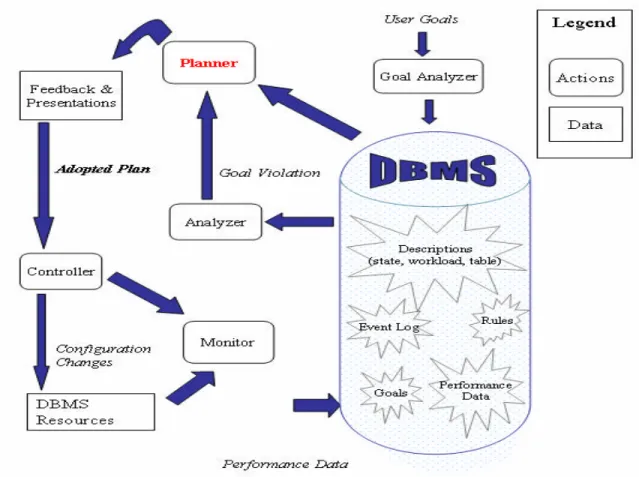
The diagnosis system is designed to fit into Quartermaster, a framework for automating performance management of DBMS systems [BEN99] [MAR00]. Quartermaster supports the collection and storage of performance data and the monitoring of performance goals. An overview of the Quartermaster framework is presented in Figure 3. The “Planner” module in the Quartermaster framework is responsible for determining the resource that should be tuned to solve a performance problem. The diagnosis framework defined in this dissertation provides the Planner module.

Resource Model Workload Model Diagnosis Tree Diagnosis Tune DBMS

DBMS Expertise and Documentation Legend Actions Data Models Resources to be Tuned Diagnostic Rules Collect Performance Data

Figure 2 – Overview of the Diagnosis Models.

(45)

Figure 3 - The Quartermaster Architecture.

3.2 Resource Model

The resource model is a collection of information about the DBMS, DBMS resources, and the relationships between those resources. Information about the resources is gathered from several different sources. DBMS manuals provide much of the information about the DBMS and resources. This information is further expanded using other DBMS documentation and technical reference books. A more in-depth view of the DBMS resources can be produced by consultation with DBMS programmers and DBAs. Consultation allows for the inclusion of undocumented information in the model. The

(46)

resource model is used to present a consolidated view of DBMS information from many sources and make this information available to for diagnosis purposes. The focus of the resource model is to establish two types of information – information about the resources and information about the relationships between the various resources. We now consider the two types of information.

3.2.1 Resources

Resources are defined as any object used by the DBMS where the amount of the object can be adjusted. Resources are further refined into two categories – physical and logical resources. Physical resources are hardware-oriented resources whose allocations have a direct effect on the physical hardware. Examples of physical resources are main memory or disk space. Allocations of physical resources are limited by the hardware available from the system for the DBMS. In general, the more physical resources available to the DBMS the better it will perform. Logical resources are those resources that are provided by the DBMS. An example of a logical resource is the number of processes allocated to write data to disk. Logical resource allocations are limited by the DBMS. Some of the limits may be indirectly linked to the amount of physical resources available (such as the DBMS denying the creation of a process due to a lack of memory). Logical resource allocations do have an effect on physical resources, as the DBMS must use memory and CPU to maintain these processes. Some logical resources, such as the number of I/O processes, will also have an affect on system resources such as disk drive performance.

(47)

In our model, a resource in the DBMS has the following attributes:

• Impact – The impact that this resource has on DBMS performance. Impact is categorized as either high, medium or low. High impact resources will have a greater effect on performance than low impact resources.

• Allowable range – The allowable (legal) range of values that the resource may be assigned. Lower and upper limits of the range are specified by the DBMS documentation. The allowable range of resource values is strictly a software or hardware limitation; the allowable range is not based on performance.

• Default value – The default value assigned to the resource by the DBMS.

• Marker values – A list of marker names and values. Markers are observed or calculated values that can be used to determine how the system is performing with respect to the resource in question.

• Setting values – A list of setting values associated with the resource. A single resource may be associated with several tuning parameters. A setting value is a tuning parameter and its current value.

A resource can be represented by a single tuple

R = <M, I, <S, A>, D>

where M = {M1, M2, …, Mn}; Mi is a marker of the form <mname, mvalue>; I is the

impact that the particular resource has on performance; <S, A> = a set of tuples <Si, Ai>

where Si is a setting of the form <sname, svalue> and Ai is the range of possible values

(48)

This formal resource definition is used to create the ER diagram of a resource (shown in Figure 4), which is the basis of the relational model used for our specific implementation.

1

Resource

Marker

Impact

Default Value

Value

Name

Range

Setting

has

1 m

Figure 4 - ER diagram of the formal resource definition.

An example of a DB2 database resource is the number of Input/Output (I/O) cleaner processes allocated in the DBMS. The I/O Cleaners can be expressed in the tuple:

num_iocleaners = < <% of async writes, 95>, <num_iocleaners, 10, {0-255}>, HIGH, 1> In this example, the marker value used to determine the performance of the number of I/O cleaners resource is the percentage of asynchronous writes made by the DBMS. If the percentage of asynchronous writes is low, then the I/O cleaners are not properly writing dirty pages back to disk and slower synchronous writes are being used. The setting va lue used in this example is 10, signifying the number of I/O cleaners presently allocated in the DBMS. Increasing the number of I/O cleaners will increase concurrency but may

(49)

overload a system that cannot handle more concurrency. The impact of the I/O cleaners resource on the DBMS has been rated as HIGH by the documentation. The HIGH rating signifies that adjusting this resource can have a significant impact on the performance of the system. The range of legal values for the I/O cleaners resource is between 0 and 255. The DBMS software will allow a DBA to specify anywhere from 0 I/O cleaner processes to 255 I/O cleaner processes. Internal structures in the DBMS will not allow more I/O cleaners to be allocated, limiting the maximum number of I/O cleaners in the system. We are allowed to specify a lower number of 0 I/O cleaners for the situation where the database is read-only, removing the need to write updates back to the database and rendering the I/O cleaner processes unneeded. The final attribute for the I/O cleaner resource is the default value used by IBM when the DBMS is initially installed. The default value for this resource is 1, indicating that a single I/O cleaner process will be allocated under the default settings. We store the default DBMS resource settings as a reference point to an out-of-the-box resource allocation. All of the information used to define the tuple for the I/O cleaner resource was extracted from DB2 documentation and experience using DB2.

3.2.2 Resource Relationships

Key data required for the construction of the resource model pertains to the relationships between various DBMS resources. Relationship information is critical because adjusting the value of one resource will have an effect on those resources that are closely related to it. Information about resource relationships can be extracted from DBMS documentation or from DBA experience. DB2 documentation specifies the relationship between various

(50)

resources. Consider, for example, the I/O cleaners resource. Documentation for DB2 specifies that if the number of I/O cleaners is modified, we should also consider adjusting the related parameters buffer pool size and changed pages threshold. Buffer pool size is the amount of cache memory that we have allocated for use by the DBMS. Changed Pages Threshold is the percentage of updated pages required in the buffer pool before the I/O cleaner processes are started to write the changed pages back to disk.

Determining the relationships between various resources is important for DBMS diagnosis. Knowing that adjusting one resource may have an effect on other resources allows us to make a more knowledgeable decision when diagnosing the DBMS. It should be noted that resource relationship information is directional. DB2 documentation suggests that while adjusting the buffer pool size we should also consider adjusting the changed pages threshold parameter, but while adjusting the changed pages threshold the documentation does not recommend adjusting the size of the buffer pool.

The resource model can be represented by the set RM = {<R, {E}>}

where in each tuple of the set, R in the set is a resource and E = {E1, E2, … Ei}; Ei is a

directed edge from that resource to another resource in the resource model. A directed edge from Ri to Rj indicates that a change in resource Ri can have a direct effect on

resource Rj. The resource model is visually represented as a directed graph. It is possible

to have two edges between a pair of nodes – one in each direction. We simplify our resource model by reducing these pairs of edges to a single edge with arrows on both

(51)

ends. Relationship information must be gathered before the resource model is constructed. Collecting resource relationship information is a one-time task for a DBMS. The ER diagram for the resource model is shown in Figure 5. This ER model is the basis for our relational implementation. Figure 6 is an example resource model.

Resource has Edge

rName

n m

Figure 5 - ER diagram of the resource model.

Buffer Pool Size LockList Size

Log Buffer Size Catalog Cache Size

Database Heap Size

Changed Pages Threshold Lock Timeout

Maxlocks

Sort Heap Threshold

Sort Heap Size

Max Number of Agents

Application Heap Size Max Number of Applications

Application Control Heap Size

Number of I/O Cleaners Deadlock Check Time

Average Num of Applications

(52)

3.2.3 Generating Resource Subtrees

The resource model is used to store information about relationships between various resources in the DBMS. The considerable size of the resource model makes it beneficial to generate smaller resource trees when dealing with a DBMS resource. Smaller resource trees are used to simplify resource information for a given resource. The smaller resource “subtrees” can be used during the diagnosis process. Cycles from the original resource model are removed during the generation of the smaller resource subtrees. Eliminating cycles from the graph removes the possibility of a resource occurring in the subtree multiple times.

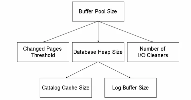
The resource model stores directional information relating to the impact of one resource on another. Knowing that one resource has an impact on another resource allows us to predict the impact of adjusting each DBMS resource. For each resource adjusted in the DBMS, we can determine the “ripple effect” this adjustment will have on other resources in the system. This allo ws us to predict the effects of resource adjustment. To predict the effects of resource adjustment, we can generate a forward resource tree. A forward resource tree will have, as the root node, the resource that is to be adjusted. Each node in the forward resource tree that is one edge away from the root will be directly affected by an adjustment of the root resource. A forward resource tree can be generated as many levels deep as desired, further determining the effect of adjusting the resource at the root of the tree.

(53)

Forward resource trees are generated by first determining a node to act as the root of the forward resource tree. Next, all of the resources that are directly affected by the root node are included in the forward resource tree, with arrows pointing from the root node to each node added to the tree. Each of these new nodes is a “Level 1” node. For each individual resource in Level 1, we determine all of the resources that are directly affected by that individual resource and include them in the tree as part of “Level 2”, with arrows from the Level 1 resource to these new resources. It should be noted that any individual resource should only appear in a forward resource tree once, eliminating circular references. Duplicate resource nodes should be ignored and not included in the forward resource tree. After this process has been completed for all of the nodes in Level 1, then a full forward resource tree will have been generated to two levels. If further levels are desired, all of the nodes in Level 2 can be examined and new resource nodes can be added to create Level 3. A sample forward resource tree is found in Figure 7. The forward resource tree in Figure 7 is generated from the resource model example in Figure 6 with the Buffer Pool Size as the root node. The forward resource tree in Figure 7 is generated to a depth of two.

(54)

Figure 7 - An example of a generated forward resource tree.

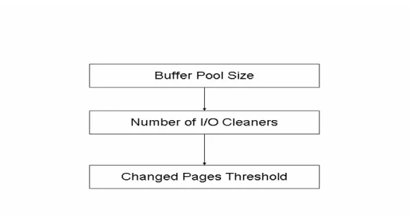
Although the forward resource trees are useful for determining the effects of adjusting a particular resource, they do not help in determining which resource settings may cause another resource to perform poorly. For example, assume that the buffer pool resource is chosen for adjustment by a diagnosis algorithm. It may be beneficial for both the diagnosis and tuning algorithms to know which resource adjustments may have caused the buffer pool resource to perform poorly. To determine which resources may have affected the buffer pool resource, we generate a reverse resource tree. A reverse resource tree has the selected resource as the root. Each node one edge away from the root is a resource that, if adjusted, will have an effect on the root resource. By generating a reverse resource tree, it is possible to determine if the root cause of the performance problem is actually the resource at the root node or another resource that is causing the resource at the root node to behave poorly. Reverse resource trees are also effective in that if we have multiple resources that are being considered for tuning, it is possible to

(55)

compare reverse resource trees to see if the resources have a resource in common that may be affecting the resources considered for tuning. Figure 8 is an example of a reverse resource tree with the buffer pool resource as the root node.