M E T H O D O L O G Y
Open Access
Missing data approaches for probability
regression models with missing outcomes
with applications
Li Qi and Yanqing Sun
**Correspondence: [email protected] Department of Mathematics and Statistics, The University of North Carolina at Charlotte, 28223 Charlotte, NC, USA
Abstract
In this paper, we investigate several well known approaches for missing data and their relationships for the parametric probability regression modelPβ(Y|X)when outcome of interestYis subject to missingness. We explore the relationships between the mean score method, the inverse probability weighting (IPW) method and the augmented inverse probability weighted (AIPW) method with some interesting findings. The asymptotic distributions of the IPW and AIPW estimators are derived and their efficiencies are compared. Our analysis details how efficiency may be gained from the AIPW estimator over the IPW estimator through estimation of validation probability and augmentation. We show that the AIPW estimator that is based on augmentation using the full set of observed variables is more efficient than the AIPW estimator that is based on augmentation using a subset of observed variables. The developed
approaches are applied to Poisson regression model with missing outcomes based on auxiliary outcomes and a validated sample for true outcomes. We show that, by stratifying based on a set of discrete variables, the proposed statistical procedure can be formulated to analyze automated records that only contain summarized
information at categorical levels. The proposed methods are applied to analyze influenza vaccine efficacy for an influenza vaccine study conducted in Temple-Belton, Texas during the 2000-2001 influenza season.
Mathematics Subject Classification: Primary 62J02; Secondary 62F12
Keywords: Augmented inverse probability weighted estimator; Asymptotic results; Automated records; Auxiliary outcome; Efficiency; Inverse probability weighted estimator; Mean score estimation; Recurrent events; Vaccine efficacy; Validation sample
1 Introduction
Suppose thatYis the outcome of interest andXis a covariate vector. One is often inter-ested in the probability regression modelPβ(Y|X)that relatesY toX. In many medical and epidemiological studies, the complete observations onYmay not be available for all study subjects because of time, cost, or ethical concerns. In some situations, an easily measured but less accurate outcome named auxiliary outcome variable, A, is supple-mented. The relationship between the true outcomeYand the auxiliary outcomeAin the available observations can inform about the missing values ofY. LetV be a subsample of
the study subjects, termed the validation sample, for which both true and auxiliary out-comes are available. Thus observations on(X,Y,A)are available for the subjects inVand only(X,A)are observed for those not inV.
It is well known that the complete-case analysis, which uses only subjects who have all variables observed, can be biased and inefficient, cf. Little and Rubin (2002). The issues also rise when substituting auxiliary outcome for true outcome; see Ellenberg and Hamilton (1989), Prentice (1989) and Fleming (1992). Inverse probability weighting (IPW) is a statistical technique developed for surveys by Horvitz and Thompson (1952) to calculate statistics standardized to a population different from that in which the data was collected. This approach has been generalized to many aspects of statistics under various frameworks. In particular, the IPW approach is used to account for missing data through inflating the weight for subjects who are underrepresented due to missingness. The method can potentially reduce the bias of the complete-case estimator when weighting is correctly specified. However, this approach has been shown to be inefficient in sev-eral situations, see Clayton et al. (1998) and Scharfstein et al. (1999). Robins et al. (1994) developed an improved augmented inverse probability weighted (AIPW) complete-case estimation procedure. The method is more efficient and possesses double robustness property. The multiple imputation described in Rubin (1987) has been routinely used to handle missing data. Carpenter et al. (2006) compared the multiple imputation with IPW and AIPW, and found AIPW as an attractive alternative in terms of double robustness and efficiency. Using the maximum likelihood estimation (MLE) coupled with the EM-algorithm (Dempster et al. 1977), Pepe et al. (1994) proposed the mean score method for the regression modelPβ(Y|X)when bothXandAare discrete.
In this paper, we investigate several well known approaches for missing data and their relationships for the parametric probability regression modelPβ(Y|X)when out-come of interest Y is subject to missingness. We explore the relationships between the mean score method, IPW and AIPW with some interesting findings. Our analy-sis details how efficiency is gained from the AIPW estimator over the IPW estimator through estimation of validation probability and augmentation to the IPW score func-tion. Applying the developed missing data methods, we derive the estimation procedures for Poisson regression model with missing outcomes based on auxiliary outcomes and a validated sample for true outcomes. Further, we show that the proposed sta-tistical procedures can be formulated to analyze automated records that only contain aggregated information at categorical levels, without using observations at individual levels.
of the main results are given in the Appendix A, while the proof of a simplified variance formula in Section 4 is placed in the Appendix B.
2 Missing data approaches
Consider the probability regression modelPβ(Y|X), whereY is the outcome of interest andXis a covariate vector. LetAbe the auxiliary outcome forYandVbe the validation set such that observations on(X,Y,A)are available for the subjects inVand only(X,A) are observed for those inV¯, the complement ofV. In practice, the validation sample may be selected based on the characteristics of a subset,Z, of the covariates inX. We writeX= (Z,Zc). For example,Zmay include exposure indicator and other discrete covariates and Zcmay be the exposure time. Let(Zi,Xi,Yi,Ai),i= 1,. . .,n, be independent identically distributed (iid) copies of(Z,X,Y,A). Letξi=I(i∈V)be the selection indicator.
Most statistical methods for missing data require some assumptions on missingness mechanisms. The commonly used ones are missing completely at random (MCAR) and missing at random (MAR). MCAR assumes that the probability of missingness in a variable is independent of any characteristics of the subjects. MAR assumes that the probability that a variable is missing depends only on observed variables. In practice, if missingness is a result by design, it is often convenient to let the missing probability depend on the categorical variables only. There is also simplicity in statistical inference by modeling the missing probability based on the categorical variables. We introduce the following missing at random assumptions.
MAR I: ξiis independent ofYiconditional on(Xi,Ai)andξiis independent ofZci
conditional on(Zi,Ai).
MAR II: ξiis independent of(Yi,Zic)conditional on(Zi,Ai).
Since the conditional density f(y,zc|ξ,z,a) = f(zc|ξ,z,a)f(y|zc,ξ,z,a) = f(zc|z,a) f(y|zc,z,a) = f(y,zc|z,a), MAR I implies MAR II. It is also easy to show that MAR II implies MAR.
Let πˆi be the estimator of the conditional probability πi = P(ξi = 1|Xi,Ai), and ˆ
πz
i the estimator of πiz = P(ξi = 1|Zi,Ai). Let Sβ(Y|X) denote the partial deriva-tives of logPβ(Y|X) with respect to β. Let EˆSβ(Y|Xi)|Xi,Ai
be the estimator of the conditional expectation ESβ(Y|Xi)|Xi,Ai
, and EˆSβ(Y|Xi)|Zi,Ai
the estimator of ESβ(Y|Xi)|Zi,Ai. We investigate several estimators of β based on the following estimating equations with different choices ofWi:
n
i=1
Wi=0, (1)
whereWitakes one of the following forms:
WiI1= ξi
ˆ
πz i
Sβ(Yi|Xi) (2)
WiE1=ξiSβ(Yi|Xi)+(1−ξi)Eˆ
Sβ(Y|Xi)|Zi,Ai
(3)
WiA1= ξi
ˆ
πz i
Sβ(Yi|Xi)+
1− ξi
ˆ
πz i
ˆ
ESβ(Y|Xi)|Zi,Ai
(4)
WiI2= ξi
ˆ
πi
WiE2=ξiSβ(Yi|Xi)+(1−ξi)Eˆ
Sβ(Y|Xi)|Xi,Ai
(6)
WiA2= ξi
ˆ
πz i
Sβ(Yi|Xi)+
1− ξi
ˆ
πz i
ˆ
ESβ(Y|Xi)|Xi,Ai
. (7)
WiA3= ξi
ˆ
πi
Sβ(Yi|Xi)+
1− ξi
ˆ
πi
ˆ
ESβ(Y|Xi)|Xi,Ai. (8)
The estimatorβˆI1obtained by usingWiI1is an IPW estimator where a subject’s valida-tion probabilityπizdepends only on the category defined by(Zi,Ai). BecauseE
(πz i)−1ξi Sβ(Yi|Xi)
=ESβ(Yi|Xi)
=0, the estimatorβˆI1is approximately unbiased. The estima-torβˆI2obtained by usingWiI2is also an IPW estimator but with the validation probability πidepending on the category defined by(Zi,Ai)and the additional covariateZci.
The estimatorβˆE1obtained by usingWiE1is the mean score estimator where the scores Sβ(Yi|Xi) for those with missing outcomes are replaced by the estimated conditional expectations given(Zi,Ai). The estimatorβˆE2obtained by usingWiE2is the mean score estimator where the scoresSβ(Yi|Xi)for those with missing outcomes are replaced by the estimated conditional expectations given(Xi,Ai). The estimatorβˆE2is the mean score estimator in Pepe et al. (1994). The mean score estimator is the MLE estimator employing the EM-algorithm (Dempster et al. 1977) under the assumption that the auxiliary out-come is noninformative in the sense that the probability modelPθ(A|Y,X)is unrelated to β.
The estimatorβˆA1 obtained using WiA1 is the AIPW estimator augmented with the estimated conditional expectationEˆSβ(Y|Xi)|Zi,Ai
. The estimatorβˆA2obtained using WiA2 is the AIPW estimator augmented with the estimated conditional expectation
ˆ
ESβ(Y|Xi)|Xi,Ai. The estimatorβˆA3is obtained usingWiA3. TheWiA3differs fromWiA2 in that the estimated validation probability isπˆiinstead ofπˆiz.
Suppose that πˆiz is an asymptotically unbiased estimator of π¯iz and that
ˆ
ESβ(Y|Xi)|Zi,Ai
is asymptotically unbiased ofE¯Sβ(Y|Xi)|Zi,Ai
, where bothπ¯izand
¯
ESβ(Y|Xi)|Zi,Ai
are functions of (Zi,Ai). Under MAR II, if one of the equalities, ¯
πz
i =πizandE¯
Sβ(Y|Xi)|Zi,Ai
=ESβ(Y|Xi)|Zi,Ai
, holds, then
E π¯iz−1ξiSβ(Yi|Xi)
+E 1−πiz−1ξi
¯
ESβ(Y|Xi)|Zi,Ai
=ESβ(Yi|Xi)
=0,
which entails that the estimatorβˆA1has the double robust property in the sense that it is a consistent estimator ofβif eitherπˆizis a consistent estimator ofπizorEˆSβ(Y|Xi)|Zi,Ai
is a consistent estimator ofESβ(Y|Xi)|Zi,Ai. Similarly, under MAR I, the estimator ˆ
βA2 possesses the double robust property in thatβˆA2is a consistent estimator of β if eitherπˆizis a consistent estimator ofπizorEˆSβ(Y|Xi)|Xi,Ai
is a consistent estimator of ESβ(Y|Xi)|Xi,Ai
. The estimatorβˆA3has similar double robust property asβˆA2.
3 Method comparisons and asymptotic results
conditional expectationESβ(Y|Xi)|Xi,Ai
can be nonparametrically estimated based on the validation sample,
ˆ
ESβ(Y|Xi)|Xi,Ai=
j∈V(Xi,Ai)
SβYj|Xj/nV(Xi,Ai), (9)
Under MAR I,EˆSβ(Y|Xi)|Xi,Ai
is an unbiased estimator ofESβ(Y|Xi)|Xi,Ai
. Now we letV(Zi,Ai)denote the subjects inVwith values of(Z,A)equal to(Zi,Ai),nV(Zi,Ai) the number of subjects inV(Zi,Ai), andn(Zi,Ai)the number of subjects in the sample with values of(Z,A)equal to(Zi,Ai). A nonparametric estimator ofπiz=P(ξi=1|Zi,Ai) is given byπˆiz=nV(Z
i,Ai)/n(Zi,Ai). A nonparametric estimator ofE{Sβ(Y|Xi)|Zi,Ai}is given by
ˆ
ESβ(Y|Xi)|Zi,Ai
=
j∈V(Zi,Ai)
SβYj|Xj
/nV(Zi,Ai). (10)
Under MAR II, (Yi,Xi) is independent of ξi conditional on (Zi,Ai), then ˆ
ESβ(Y|Xi)|Zi,Ai
is an unbiased estimator ofE{Sβ(Y|Xi)|Zi,Ai}.
Proposition 1. Suppose that X =(Z,Zc)and A are discrete and their dimensionality is reasonably small. Under the nonparametric estimatorsπˆiz = nV(Zi,Ai)/n(Zi,Ai),πˆi = nV(Xi,Ai)/n(Xi,Ai)and the estimators for the conditional expectation defined in (9) and (10), the estimatorsβˆI1,βˆE1andβˆA1are equivalent, and the estimatorsβˆI2,βˆE2,βˆA2and
ˆ
βA3are equivalent. However, the estimatorβˆA2is different fromβˆA1unless Zci is linearly related to Ziin which caseβis not identifiable.
The results of Proposition 1 are very intriguing since research has shown that the AIPW and the mean score methods are more efficient than the IPW method. It is also intriguing that the AIPW estimatorsβˆA2andβˆA3are actually the same estimators, not affected by the validation probability. To further understand these approaches, we investi-gate the asymptotic properties of these methods where(X,A)are not necessarily discrete. Through the asymptotic analysis, we gain insights about what matters to the efficiency in terms of the selections of the validation sample and the augmentation function.
Suppose that E˜Sβ(Y|Xi)|Xi,Ai
is a consistent parametric/nonparametric estima-tor ofEa
Sβ(Y|Xi)|Xi,Ai
, whereEa
Sβ(Y|Xi)|Xi,Ai
isESβ(Y|Xi)|Xi,Ai
orE{Sβ(Y| Xi)|Zi,Ai}. Let π(Xi,Ai,ψ) be the parametric model for the validation probability πi, whereψ is aq-dimensional parameter. We show in Corollary 2 that the nonparametric estimator ofπ(Xi,Ai,ψ)can also be expressed in the parametric form when(Xi,Ai)are discrete. Letψ0 be the true value ofψ. Under MAR I, the MLE ψˆ =
ˆ
ψ1,. . .,ψˆq
of ψ =(ψ1,. . .,ψq)is obtained by maximizing the observed data likelihood,
n
i=1
{π(Xi,Ai,ψ)}ξi{1−π(Xi,Ai,ψ)}1−ξi.
The validation probabilityπiis estimated byπ˜i = π
Xi,Ai,ψˆ
. Then by the standard likelihood based analysis, we have the approximation
ˆ
ψ−ψ0=n−1 n
i=1
Iψ−1Sψi +op
whereSψi andIψare the score vector and information matrix forψˆ defined by
Siψ = (ξi−π(Xi,Ai,ψ0)) π(Xi,Ai,ψ0)(1−π(Xi,Ai,ψ0))
∂π(Xi,Ai,ψ0)
∂ψ ,
Iψ = E
1
π(Xi,Ai,ψ0)(1−π(Xi,Ai,ψ0)) ∂π(
Xi,Ai,ψ0) ∂ψ
⊗2
, (12)
wherea⊗2=aa.
Consider the IPW estimatorβˆIobtained by solving the estimating equation
UI= n
i=1 ξi ˜
πi
Sβ(Yi|Xi) (13)
and the AIPW estimatorβˆAbased on solving the estimating equation
UA= n
i=1 ξ
i ˜
πi
Sβ(Yi|Xi)+
1− ξi
˜
πi
˜
ESβ(Y|Xi)|Xi,Ai
. (14)
Theorem 1. Assume that Pβ(Y|X)andπ(X,A,ψ)have bounded third-order derivatives in a neighborhood of the true parameters and are bounded away from 0 almost surely, both −E∂2/∂β2 logPβ(Y|X) and Iψ are positive definite at the true parameters. Then, underMAR I,
n1/2
ˆ
βI−β
=I−1(β)n−1/2 n
i=1
QIi+op(1),
n1/2βˆA−β
=I−1(β)n−1/2 n
i=1
QAi +op(1),
where I(β)=E−∂2/∂β2 logPβ(Y|X)=VarSβ(Yi|Xi)
,
QIi =ξi/πiSβ(Yi|Xi)−E
πi−2ξiSβ(Yi|Xi) (∂π(Xi,Ai,ψ0)/∂ψ)
(Iψ)−1Sψi
and QAi =ξi/πiSβ(Yi|Xi)+(1−ξi/πi)Ea
Sβ(Y|Xi)|Xi,Ai
. Both n1/2
ˆ
βI−β
and n1/2
ˆ
βA−β
have asymptotically normal distributions with mean zero and covariances equal to I−1(β)VarQIiI−1(β)and I−1(β)VarQAi I−1(β), respectively. Further,
VarQIi=VarQiA+Var(Bi+Oi) (15)
and
Var
QAi
=I(β)+Var
1− ξi πi
Sβ(Yi|Xi)−Ea
Sβ(Y|Xi)|Xi,Ai
, (16)
where Oi = E
πi−2ξiSβ(Yi|Xi) (∂π(Xi,Ai,ψ0)/∂ψ)
(Iψ)−1Sψi and Bi = (1−ξi/πi) Ea
Sβ(Y|Xi)|Xi,Ai
.
Suppose that the validation probability πi = P(ξi=1|Xi,Ai) depends only on (Zi,Ai). That is, πi = πiz = P(ξi=1|Zi,Ai). Suppose that π˜i is the MLE of πiz under the parametric familyψ(Zi,Ai,ψ). Let βˆA1 be the estimator obtained by solv-ing (14) where the augmented term, E˜Sβ(Y|Xi)|Xi,Ai
, is a consistent paramet-ric/nonparametric estimator ofESβ(Y|Xi)|Zi,Ai
. LetβˆA2 be the estimator obtained by solving (14) whereE˜Sβ(Y|Xi)|Xi,Ai
is a consistent parametric/nonparametric esti-mator ofESβ(Y|Xi)|Xi,Ai
(Z,A), of observed variables and the other that corresponds to the augmentation based on the full set,(X,A), of the observed variables.
Corollary 1. Suppose that the validation probabilityπi= P(ξi =1|Xi,Ai)depends only on(Zi,Ai). Under the conditions of Theorem 1,
n1/2
ˆ
βA1−β
D
−→N0,I−1(β)+I−1(β)A1(β)I−1(β)
, (17)
and
n1/2βˆA2−β
D
−→N0,I−1(β)+I−1(β)A2(β)I−1(β)
, (18)
whereA1(β)=E((1−πiz)/πiz)Var{Sβ(Yi|Xi)|Zi,Ai}andA2(β)=E((1−πiz)/πiz) VarSβ(Yi|Xi)|Xi,Ai
. The asymptotic variance ofβˆA2 is smaller than the asymptotic variance ofβˆA1if the covariates Ziare a proper subset of Xi.
Suppose that(Z,A)are discrete taking values(z,a)in a setZof finite number of values. If the number of parameters inψ equals the number of valuesψz,a = P(ξi = 1|Zi = z,Ai = a) for all distinct pairs(z,a), thenψ = {ψz,a}andπ(z,a,ψ) = ψz,a. Further,
∂π(z,a,ψ0)
∂ψ can be viewed as a column vector with 1 in the position forψz,aand 0 elsewhere. The information matrixIψdefined in (12) has the expression,
Iψ= z,a
ρ(z,a)
1
π(z,a,ψ0)(1−π(z,a,ψ0))
∂π(z,a,ψ0) ∂ψ
∂π(z,a,ψ0) ∂ψ
,
whereρ(z,a)=P(Zi =z,Ai =a). It follows thatIψ is a diagonal matrix and its inverse matrix is also diagonal. The MLEψˆz,a = nV(z,a)/n(z,a) is in fact the nonparametric estimator forψz,abased on the proportion of validated samples in the category specified by(z,a). The equation (11) can be expressed as
ˆ
ψz,a−π(z,a,ψ0)=n−1
nV(z,a)−n(z,a)π(z,a,ψ 0) ρ(z,a) +op
n−1/2,
for(z,a)∈Z.
By Threom 1, the possible efficiency gain of the AIPW estimator over the IPW estimator is shown through the equation (15). The AIPW estimator is more efficient unless Var(Bi+ Oi)=0. In particular, from the proof of Theorem 1, we have
n−1/2UA = n−1/2 n
i=1
QAi +op(1) (19)
n−1/2UI = n−1/2 n
i=1
QAi −n−1/2 n
i=1
(Bi+Oi)+op(1), (20)
whereBiandOiare defined following (16). The following corollary presents the analysis of the termn−1/2ni=1(Bi+Oi)when(Zi,Ai)are discrete to understand how efficiency may be gained from the AIPW estimator over the IPW estimator.
validation probabilityπi = P(ξi =1|Xi,Ai)only depends on(Zi,Ai)andψz,a = P(ξi = 1|Zi=z,Ai =a)is estimated nonparametrically byψˆz,a=nV(z,a)/n(z,a). Then
n−1/2 n
i=1
(Oi+Bi)
= −
z,a n−1/2
n
j=1
ξj−π(z,a,ψ0) π(z,a,ψ0)
I(Zj=z,Aj=a)
E{Sβ(Yj|Xj)|Zj=z,Aj=a} −E Sβ(Yj|Xj)|Zj=z,Zcj,Aj=a
.
(21)
By Corollary 2, (19) and (20),βˆAis more efficient thanβˆI unlessVar{Sβ(Yj|Xj)|Zj = z,Aj =a} =0 for all(z,a)for whichP(Zi =z,Ai =a)=0. IfX=Zand the validation probabilityπi=P(ξi=1|Xi,Ai)is nonparametrically estimated with the cell frequencies
ˆ
ψz,a=nV(z,a)/n(z,a), thenβˆAandβˆIare asymptotically equivalent.
RemarkConsider the estimators ofβ obtained based on the estimating equation (1) corresponding to different choices ofWigiven in (2) to (8). If(Z,A)are discrete and the validation probabilityπiz = P(ξi = 1|Zi,Ai)is estimated nonparametrically by the cell frequency, then by Theorem 1 and Corollary 2,βˆA1andβˆI1have same asymptotic normal distributions as long asE[ˆ Sβ(Y|Xi)|Zi,Ai] is a consistent estimator ofE[Sβ(Y|Xi)|Zi,Ai]. ButβˆA2is more efficient thanβˆI1as long asE[ˆ Sβ(Y|Xi)|Xi,Ai] is a consistent estimator ofE[Sβ(Y|Xi)|Xi,Ai] since Var(Bi+Oi)is not zero by (21). These results are not affected by whetherE[Sβ(Y|Xi)|Zi, Ai] andE[Sβ(Y|Xi)|Xi,Ai] are estimated nonparametrically or based on some parametric models. In addition, by Theorem 1, Corollary 1 and 2,βˆA3 andβˆI2have the same asymptotic normal distributions as long asE[ˆ Sβ(Y|Xi)|Xi,Ai] is a consistent estimator ofE[Sβ(Y|Xi)|Xi,Ai].
4 Poisson regression using the automated data with missing outcomes Many medical and public health data are available only in aggregated format, where the variables of interest are aggregated counts without being available at individual levels. Many existing statistical methods for missing data require observations at individual lev-els. Applying the missing data methods presented in Section 3, we derive some estimation procedures for the Poisson regression model with missing outcomes based on auxiliary outcomes and a validated sample for true outcomes. Further, we show that, by stratifying based on a set of discrete variables, the proposed statistical procedure can be formulated so that it can be used to analyze automated records which do not contain observations at individual levels, only summarized information at categorical levels.
LetYrepresent the number of events occurring in the time-exposure interval [0,T] and Zthe covariates. We consider the Poisson regression model,
P(Y =y|Z,T)=exp−Texp(βZ) Texp(βZ)y/y!, (22)
number of auxiliary eventsAfor MAARI is collected based on ICD-9 codes through hos-pital records. Further diagnosis may indicate that some of these events are false events. The number of true vaccine adverse events,Y, can only be confirmed for the subjects in the validation setV. Suppose thatZis the vaccination status, 1 for the vaccinated and 0 for the unvaccinated. Then, under Poisson regression, exp(β)is the relative rate of event occurrence per unit time of the exposed versus unexposed. We assume that the num-ber of automated eventsAcan be expressed asA= Y+W, whereW is the number of false events independent ofYconditional on(Z,T). Suppose thatWfollows the Poisson regression model
P(W =w|Z,T)=exp−Texp(γZ) Texp(γZ)w/w!, (23)
whereγ=a0,a1,γ1,· · ·,γk−1
.
We apply the missing data methods introduced in Section 3 on model (22). The vari-ables(Zi,Ti,Yi,Ai)are observed for the validation sampleVand(Zi,Ti,Ai)are observed for the nonvalidation sampleV. While the covariate¯ Zcan be considered as categorical, it is natural to consider the exposure timeTas a continuous variable. We assume that the validation probability depends only on the stratification of(Z,A). That is, the validation sample is a stratified random sample by the categories defined by(Z,A). Of those estima-tors discussed in Section 2, there are only two different estimaestima-tors,βˆI1andβˆA2. We show in Section 4.3 that the proposed method can be formulated so that it can be used to ana-lyze the automated records with missing outcomes. First we derive the explicit estimation procedures forβˆI1andβˆA2and their variance estimators under model (22).
4.1 Inverse probability weighting estimation
We adopt all notations introduced in Section 3. In particular, letπiz = P(ξi = 1|Zi,Ai) and πˆiz = nV(Zi,Ai)/n(Zi,Ai). LetX = (Z,T) and Xi = (Zi,Ti) to be consistent with earlier notations. The score function for subjectiunder model (22) isSβ(Yi|Xi) = Zi(Yi−Tiexp(βZi)). The estimatorβˆI1is obtained by solvingin=1(ξi/πˆiz)Sβ(Yi|Xi)=0, whereSβ(Yi|Xi) =Zi(Yi−Tiexp(γZi)). By Corollary 1,√n(βˆI1−β)converges in dis-tribution to a normal disdis-tribution with mean zero and the variance matrixI−1(β)+ I−1(β)A1(β)I−1(β), whereA1(β)=E
((1−πiz)/πiz)VarSβ(Yi|Xi)|Zi,Ai
.
The information matrix I(β) = E(ZiZiTiexp(βZi)) = zP(Zi = z)zzexp(βz) E(Ti|Zi=z)can be estimated byIˆ(β)ˆ which is obtained by replacingβwithβˆI1,P(Zi=z) by the sample proportion of the event{Zi=z}, andE(Ti|Zi=z)with the sample average exposure time for those with covariatesZi=z. The matrixA1(β)can be estimated by
ˆ
A1(β)ˆ =
a,z ˆ
ρ(a,z)1− ˆρ v(a,z) ˆ
ρv(a,z) Var{Sβ(Y|X)|A=a,Z=z}, (24)
where ρ(ˆ a,z) is the estimator of P{Ai = a,Zi = z}, ρˆv(a,z) is the estimator of P{i ∈ V|Ai = a,Zi = z}, and Var
Sβ(Y|X)|A=a,Z=z is an estimator of VarSβ(Yi|Xi)|Zi,Ai
which is derived in the following.
not depend on T, the outcome Y and T are conditionally independent given(A,Z). Therefore, VarSβ(Y|X)|A,Z=ZZVar(Y|A,Z)+exp(2βZ)Var(T|A,Z). The vari-ance Var(Y|A = a,Z = z) can be estimated byapˆz(1− ˆpz), where pˆz = exp(βˆz)/
exp(βˆz)+exp(γˆz)
, and Var(T|A = a,Z = z) = E(T2|A = a,Z = z)− {E(T|A = a,Z = z)}2 can be estimated nonparametrically using the first and the second sample moments conditional on each category withA=aandZ=z.
4.2 Augmented inverse probability weighted estimation
Under the assumption thatW follows the Poisson regression model (23) and is inde-pendent of Y conditional on (Z,T), ESβ(Y|X)|Z,T,A = AZexp(βexpZ)(β+expZ)(γZ) − TZexp(βZ). LetEˆSβ(Y|Xi)|Xi,Ai
be the estimator ofESβ(Y|Xi)|Xi,Ai
for a given βby substitutingγ by its estimatorγˆI1of Section 4.1. Then the estimatorβˆA2is obtained by solving
n
i=1 ξi ˆ
πz i
Sβ(Yi|Xi)+
1− ξi
ˆ
πz i
ˆ
ESβ(Y|Xi)|Xi,Ai
=0. (25)
By Corollary 1,√n(βˆA2−β)converges in distribution to a normal distribution with mean zero and the variance matrix whereI−1(β)+I−1(β)A2(β)I−1(β), whereA2(β)= E((1−πiz)/πiz)Var{Sβ(Yi|Xi)|Xi,Ai}
. The information matrixI(β) can be estimated byˆI(β)ˆ given in Section 4.1. The conditional variance VarSβ(Y|X)|Z=z,T,A=a = apz(1− pz)z⊗2 can be estimated by apˆz(1 − ˆpz), where pˆz = exp(βˆz)/(exp(βˆz) + exp(γˆz)). It follows thatA2(β)can be consistently estimated by
ˆ
A2(β)=
a,z ˆ
ρ(a,z)1− ˆρ v(a,z) ˆ
ρv(a,z) apˆz(1− ˆpz)z ⊗2,
whereρ(ˆ a,z)is the estimator ofP{Ai=a,Zi=z}andρˆv(a,z)is the estimator ofP{i ∈ V|Ai=a,Zi=z}.
4.3 Estimation using the automated data
This section formulates the missing data estimation procedure for (22) based on the auto-mated (summarized) information at categorical levels defined by relevant covariates of the model. In particular, we show thatβˆI1andβˆA2and their variance estimators can be formulated using the automated data at categorical levels.
In many applications it is convenient to writeZ = (1,Z(1),Z(2))andβ = (b0,b1,θ), where Z(1) is the treatment indicator (Z(1) = 1 for the exposed group and Z(1) = 0 for the unexposed group) and Z(2) = (η1,· · ·,ηk−1) as the other covariates, and θ = (θ1,· · ·,θk−1). For the applications involving the automated data records, we let η1,· · ·,ηk−1bek−1 dummy variables representingkgroups. Without loss of generality, we choose thekth group as the reference group,η1=1,η2=0,· · ·,ηk−1=0 for group 1,η1 = 0,η2= 1,· · ·, ηk−1= 0 for group 2, so on andη1 =0,η2= 0,· · ·, ηk−1= 0 for groupk. Thus each value ofZdenotes a category which can be represented by(l,m) forl= 0, 1 andm =1,· · ·,k. This correspondence is denoted byZ (l,m)for conve-nience. Forl =0, 1 andm= 1,· · ·,k−1, category(l,m)is defined byZwithZ(1) =l, ηm =1 andηj= 0 forj=m,j=1,. . .,k, and category(l,k)is defined byZ(1) =land
m=1,· · ·,k, whereb1k =b0+b1,b0k =b0,b1m=b0+b1+θmandb0m=b0+θmfor 1≤ m≤k−1. The parameterb1represents the log-relative rate of the exposed versus the unexposed adjusted for other factors.
The following notations are used to show that the estimators ofβ and their variance estimators can be calculated using the automated information at the categorical levels. LetV(a,l,m)denote the set of subjects inV with (A = a,Z (l,m)),V(l,m)for the set of subjects inV with (Z (l,m)),nalm for the number of subjects with (A = a, Z(l,m)),nvalmfor the number of subjects inV(a,l,m),nvlmfor the number of subjects inV(l,m),λalm = nalm/nvalm, yalm for the number of events for subjects inV(a,l,m), ylm for the number of events for subjects inV(l,m),talmfor the total exposure time for subjects with (A= a,Z (l,m)),t2,almfor the total squared exposure time for subjects with (A=a,Z(l,m)),tlmfor the total exposure time for subjects withZ (l,m),αlm for the number of automated events for subjects withZ(l,m).
Estimation withβˆI1using the automated data. The validation probabilityπizcan be estimated by 1/λalm when Ai = a, Zi (l,m). It can be shown that the estimating equation for βˆI1 is equivalent to the following nonlinear equations for {blm, for l = 0, 1,m=1,· · ·,k},
k
m=1
a∈A
yalmλalm−eblm
a∈A
talmλalm
=0,
l=0,1
a∈A
yalmλalm−eblm
a∈A
talmλalm
=0,
forl=0, 1 andm=1,. . .,k−1. Whenk>1, the equations have no explicit solutions. In the following, we show that the asymptotic variance ofβˆI1can be consistently esti-mated by only using the autoesti-mated information at categorical levels. The information matrix is a(k+1)×(k+1)symmetric matrix given by
I(β)=E(ZiZiTiexp(βZi))
= ⎡ ⎢ ⎢ ⎢ ⎢ ⎢ ⎢ ⎢ ⎣
l,mqlm km=1q1m q11+q01 · · · q1r+q0r k
m=1q1m km=1q1m q11 · · · q1r
q11+q01 q11 q11+q01 · · · 0
..
. ... ... . .. ...
q1r+q0r q1r 0 · · · q1r+q0r
⎤ ⎥ ⎥ ⎥ ⎥ ⎥ ⎥ ⎥ ⎦ ,
wherer = k−1 andqlm = E(TieblmI{individual i in category (l,m)}). The consistent estimator,ˆI(β)ˆ , ofI(β)is thus obtained by replacingqlmwith exp(bˆlm)tlm/n.
can be estimated byνa,l,m = t2,a,l,m/nalm−(talm/nalm)2. By (24) and the discussion that follows,A1(β)can be estimated by
ˆ
A1(β)ˆ =
a,l,m ˆ
ρ(a,l,m)1− ˆρ
v(a,l,m) ˆ
ρv(a,l,m) Glm{apˆlm(1− ˆplm)+νa,l,m}, (26)
whereρ(ˆ a,l,m) = nalm/n,ρˆv(a,l,m) = nvalm/nalm andGlm be the value ofGi = z⊗i 2 when subjectibelongs to the category(l,m). Hence the covariance matrix ofβˆI1can be estimated byˆI−1(β)ˆ + ˆI−1(β)ˆ ˆA1(β)ˆ Iˆ−1(β)ˆ using the automated data.
Estimation with βˆA2 using the automated data. The estimating equations (25) are equivalent to the following nonlinear equations for{blm, forl=0, 1,m=1,· · ·,k},
k
m=1
a∈A
yalmλalm−eblmtlm+ eblm eblm+edˆ1m
αlm−
a∈A
analmλalm
=0,
l=0,1
a∈A
yalmλalm−eblmtlm+ eblm eblm+edˆlm
αlm−
a∈A
analmλalm
=0,
forl=0, 1 andm=1,. . .,k−1.
Since VarSβ(Y|X)|Z(l,m),T,A=a= aplm(1−plm)Glm,A2(β)can be consis-tently estimated by
ˆ
A2(β)ˆ =
a,l,m ˆ
ρ(a,l,m)1− ˆρ
v(a,l,m) ˆ
ρv(a,l,m) apˆlm(1− ˆplm)Glm.
Hence the covariance matrix ofβˆA2can be estimated byˆI−1(β)ˆ + ˆI−1(β)ˆ ˆA2(β)ˆ Iˆ−1(β)ˆ using the automated data.
RemarkIn the special case whereρ(α,l,m)≈0 forα≥2, a much simpler formula for the variance estimator of the log relative risk can be derived. For example in the vaccine safety study, the adverse-event rate is very small. Let
wm= α0mα1m y0my1m α0my0mnv1m+α1my1mnv0m
" k
m=1
α0mα1my0mnv1m α0my0mnv1m+α1my1mnv0m
.
Then an estimate of variance ofbˆ1is given by
Var(bˆ1)=
k
m=1 w2m
1 y1m −
1 nv1m +
1 α1m +
1 y0m−
1 nv0m +
1 α0m
, (27)
which is the weighted sum of the estimated variances for the estimated log relative rate of the exposed versus the unexposed overkgroups. The details of deviation are given in the Appendix B.
5 A simulation study
a Poisson distribution with meanTexp(b0+b1Z1+θZ2)whereb0 = −0.5,b1 = −0.8 andθ = −0.6, andWfollows a Poisson distribution with meanTexp(a0+a1Z1+γZ2) wherea0= −1.3,a1= −1.1,γ = −1. We setA=Y+W.
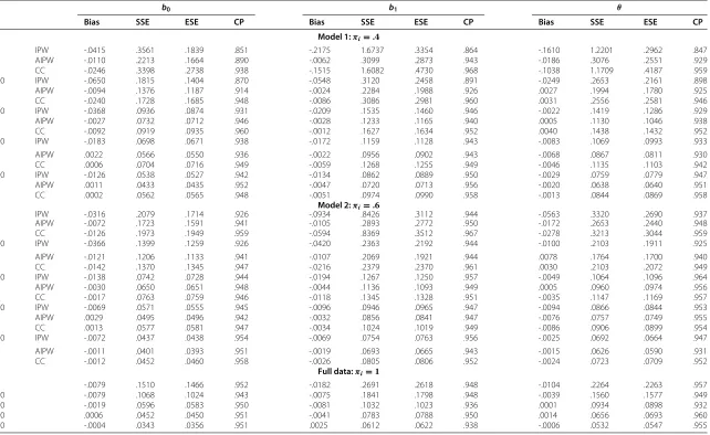
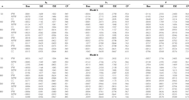
Four models for the validation sample are considered. Under Model 1, the validation sample is a simple random sample with probabilityπi =0.4. Model 2 considersπi=0.6. In Model 3, the validation probability only depends onAthrough the logistic regression model logit{πi(X,A)} =A−0.5 whereX=(Z,T). In Model 4, the validation probability depends onAandZ1through the logistic regression model logit{πi(X,A)} =A−Z1−0.5. Tables 1 and 2 present the simulation results forn = 50, 100, 300, 500 and 800. Each entry of the tables is based on 1000 simulation runs. Tables 1 and 2 summarize the bias (Bias), the empirical standard error (SSE), the average of the estimated standard error (ESE), and the empirical coverage probability (CP) of 95% confidence intervals ofβˆI1and
ˆ
βA2forβ = (b0,b1,θ). We also compare the performance of the estimatorsβˆI1andβˆA2 with the complete-case (CC) estimatorβˆCobtained by simply deleting subjects with miss-ing values ofYi. As a gold standard, we present the estimation results for the full data where all the values ofYi are fully observed. Table 1 presents the results under Model 1 and 2, and Table 2 shows the results under Model 3 and 4.
Table 1 shows that under Model 1 and Model 2, the bias of all estimators is very small at a level comparable with that of the full data estimator. The bias decreases with increased sample size and the increased level of the validation probability. The empirical standard errors are in good agreement with the corresponding estimated standard errors, except for the IPW estimator whenn≤100 andπ ≤0.6. Among them, AIPW has the smallest standard errors for all parameters and sample sizes concerned. The coverage probabilities of the confidence intervals for b0, b1 andθ are close to the nominal level 95%. When the sample size and the validation probability are both small, for example,n = 50 and π=0.4, the IPW has large bias and is unstable but the AIPW still performs well.
Table 2 gives the results under Model 3 and Model 4. The bias remains small forβˆI1and ˆ
βA2. The empirical standard errors are also close to the corresponding estimated standard errors. The coverage probabilities remain close to the nominal level 95% for all IPW and AIPW estimators. However, the complete-case estimator yields larger bias and incorrect coverage probability because of the association between the validation probability and the auxiliary variableAand/or the covariateZ1, in which case the missing is not missing completely at random. The AIPW performs better than IPW with smaller standard errors.
6 An Application
Journal
o
fStatistical
Distributions
a
nd
Applications
2014,
1
:23
Page
14
of
26
Table 1 Simulation comparison of the IPW estimatorβˆI1, the AIPW estimatorβˆA2and the complete-case (CC) estimatorβˆCunder various sample sizes and selection
probabilities
b0 b1 θ
n Bias SSE ESE CP Bias SSE ESE CP Bias SSE ESE CP
Model 1:πi=.4
50 IPW -.0415 .3561 .1839 .851 -.2175 1.6737 .3354 .864 -.1610 1.2201 .2962 .847
AIPW -.0110 .2213 .1664 .890 -.0062 .3099 .2873 .943 -.0186 .3076 .2551 .929
CC -.0246 .3398 .2738 .938 -.1515 1.6082 .4730 .968 -.1038 1.1709 .4187 .959
100 IPW -.0650 .1815 .1404 .870 -.0548 .3120 .2458 .891 -.0249 .2653 .2161 .898
AIPW -.0094 .1376 .1187 .914 -.0024 .2284 .1988 .926 .0027 .1994 .1780 .925
CC -.0240 .1728 .1685 .948 -.0086 .3086 .2981 .960 .0031 .2556 .2581 .946
300 IPW -.0368 .0936 .0874 .931 -.0209 .1535 .1460 .946 -.0022 .1419 .1286 .929
AIPW -.0027 .0732 .0712 .946 -.0028 .1233 .1165 .940 .0005 .1130 .1046 .938
CC -.0092 .0919 .0935 .960 -.0012 .1627 .1634 .952 .0040 .1438 .1432 .952
500 IPW -.0183 .0698 .0671 .938 -.0172 .1159 .1128 .943 -.0083 .1069 .0993 .933
AIPW .0022 .0566 .0550 .936 -.0022 .0956 .0902 .943 -.0068 .0867 .0811 .930
CC .0006 .0704 .0716 .949 -.0059 .1268 .1255 .949 -.0046 .1135 .1103 .942
800 IPW -.0126 .0538 .0527 .942 -.0134 .0862 .0889 .950 -.0029 .0759 .0779 .947
AIPW .0011 .0433 .0435 .952 -.0047 .0720 .0713 .956 -.0020 .0638 .0640 .951
CC .0002 .0562 .0565 .948 -.0051 .0974 .0990 .958 -.0013 .0844 .0869 .958
Model 2:πi=.6
50 IPW -.0316 .2079 .1714 .926 -.0934 .8426 .3112 .944 -.0563 .3320 .2690 .937
AIPW -.0072 .1723 .1591 .941 -.0105 .2893 .2772 .950 -.0172 .2653 .2440 .948
CC -.0126 .1973 .1949 .959 -.0594 .8369 .3512 .967 -.0278 .3213 .3044 .959
100 IPW -.0366 .1399 .1259 .926 -.0420 .2363 .2192 .944 -.0100 .2103 .1911 .925
AIPW -.0121 .1206 .1133 .941 -.0107 .2069 .1921 .944 .0078 .1764 .1700 .940
CC -.0142 .1370 .1345 .947 -.0216 .2379 .2370 .961 .0030 .2103 .2072 .949
300 IPW -.0138 .0742 .0728 .944 -.0194 .1267 .1250 .957 -.0049 .1064 .1096 .964
AIPW -.0030 .0650 .0651 .948 -.0044 .1136 .1093 .949 .0005 .0960 .0974 .956
CC -.0017 .0763 .0759 .946 -.0118 .1345 .1328 .951 -.0035 .1147 .1169 .957
500 IPW -.0069 .0571 .0555 .945 -.0096 .0946 .0965 .947 -.0094 .0866 .0844 .953
AIPW .0029 .0495 .0496 .942 -.0032 .0856 .0841 .947 -.0076 .0757 .0749 .955
CC .0013 .0577 .0581 .947 -.0034 .1024 .1019 .949 -.0086 .0906 .0899 .954
800 IPW -.0072 .0437 .0438 .954 -.0069 .0754 .0763 .956 -.0025 .0692 .0664 .947
AIPW -.0011 .0401 .0393 .951 -.0019 .0693 .0665 .943 -.0015 .0626 .0590 .931
CC -.0012 .0452 .0460 .958 -.0026 .0805 .0806 .952 -.0024 .0723 .0709 .952
Full data:πi=1
50 -.0079 .1510 .1466 .952 -.0182 .2691 .2618 .948 -.0104 .2264 .2263 .957
100 -.0079 .1068 .1024 .943 -.0075 .1841 .1798 .948 -.0039 .1560 .1577 .949
300 -.0019 .0596 .0583 .950 -.0081 .1032 .1023 .936 .0001 .0934 .0898 .932
500 .0006 .0452 .0450 .951 -.0041 .0783 .0788 .950 .0014 .0656 .0693 .960
Journal
o
fStatistical
Distributions
a
nd
Applications
2014,
1
:23
Page
15
of
26
Table 2 Simulation comparison of the IPW estimatorβˆI1, the AIPW estimatorβˆA2and the complete-case (CC) estimatorβˆCunder various sample sizes and selection
probabilities
b0 b1 θ
n Bias SSE ESE CP Bias SSE ESE CP Bias SSE ESE CP
Model 3
50 IPW .0081 .1609 .1502 .949 -.0034 .5535 .2790 .954 -.0116 .2592 .2400 .963
AIPW -.0070 .1543 .1486 .950 -.0134 .2715 .2690 .958 -.0185 .2364 .2330 .955
CC .0230 .1529 .1504 .938 .0798 .5441 .2835 .940 .0648 .2367 .2414 .952
100 IPW -.0052 .1145 .1077 .948 -.0001 .2073 .2014 .959 .0030 .1789 .1724 .948
AIPW -.0124 .1077 .1041 .947 -.0085 .1869 .1840 .957 .0050 .1636 .1606 .948
CC .0221 .1074 .1054 .939 .1023 .1830 .1937 .924 .0828 .1625 .1664 .915
300 IPW -.0011 .0617 .0614 .951 -.0044 .1176 .1157 .952 .0019 .1009 .0993 .953
AIPW -.0023 .0582 .0588 .956 -.0051 .1056 .1036 .954 .0022 .0936 .0910 .944
CC .0295 .0577 .0596 .924 .1051 .1070 .1095 .824 .0823 .0925 .0946 .861
500 IPW .0018 .0451 .0473 .958 -.0037 .0853 .0895 .958 -.0069 .0765 .0767 .945
AIPW .0009 .0430 .0452 .957 -.0032 .0793 .0798 .947 -.0066 .0689 .0702 .951
CC .0317 .0429 .0459 .903 .1077 .0788 .0844 .763 .0737 .0704 .0730 .839
800 IPW -.0006 .0374 .0375 .951 -.0030 .0671 .0708 .962 .0004 .0617 .0605 .946
AIPW -.0003 .0362 .0358 .949 -.0031 .0623 .0631 .954 -.0012 .0577 .0554 .935
CC .0315 .0353 .0364 .863 .1065 .0630 .0667 .633 .0786 .0568 .0576 .721
Model 4
50 IPW .0053 .1627 .1504 .948 .0825 .3531 .2832 .913 -.0057 .2736 .2405 .948
AIPW -.0085 .1549 .1489 .950 -.0122 .2746 .2752 .966 -.0138 .2395 .2340 .961
CC .2295 .2640 .0855 .531 .4513 .3805 .1760 .517 .2954 .3285 .1409 .536
100 IPW -.0050 .1168 .1085 .939 .0481 .2350 .2130 .922 .0016 .1884 .1761 .940
AIPW -.0130 .1083 .1043 .943 -.0067 .1920 .1885 .950 .0066 .1648 .1613 .949
CC .0196 .1077 .1063 .943 .2010 .1946 .2087 .820 .0900 .1645 .1702 .910
300 IPW -.0001 .0630 .0624 .945 -.0001 .1323 .1311 .955 -.0011 .1043 .1038 .946
AIPW -.0020 .0588 .0588 .951 -.0052 .1095 .1059 .952 .0012 .0950 .0913 .931
CC .0271 .0582 .0601 .930 .2020 .1060 .1173 .576 .0894 .0939 .0965 .863
500 IPW .0012 .0457 .0480 .951 -.0007 .0966 .1010 .966 -.0054 .0801 .0799 .948
AIPW .0006 .0433 .0453 .956 -.0010 .0821 .0813 .941 -.0059 .0697 .0704 .950
CC .0291 .0434 .0463 .912 .2047 .0817 .0903 .364 .0815 .0711 .0745 .820
800 IPW -.0006 .0381 .0380 .949 .0004 .0761 .0794 .967 .0000 .0636 .0630 .947
AIPW -.0002 .0362 .0359 .949 -.0016 .0640 .0641 .955 -.0014 .0574 .0555 .942
were noted, without another MAARI code, were excluded. More details about this study can be found in Halloran et al. (2003).
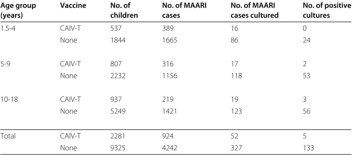
Any children representing with history of fever and any respiratory illness were eligible to have a throat swab for influenza virus culture. The decision to obtain specimens was made irrespective of whether a patient had received CAIV-T. The specific case definition was culture-confirmed influenza. Table 3 taken from Halloran et al. (2003) contains infor-mation on the number of children in three age groups, the number of children who are vaccinated versus unvaccinated, the number of nonspecific MAARI cases, the number of cultures performed, and the number of cultures positive for each group.
With the method developed in Section 4 for Poisson regression, we compare the risk of developing MAARI for children who received CAIV-T to the risk for children who had never received CAIV-T using the automated information provided in Table 3. The number of nonspecific MAARI cases extracted using the ICD-9 codes is the auxiliary outcomeA, whereas the actual number of influenza casesY is the outcome of interest. LetZ1be the treatment indicator (1=vaccine and 0=placebo). LetZ2 = (η1,η2)be the dummy variables indicating three age groups, whereη1=1 if the age is in the range 1.5– 4,η1 = 0, otherwise, andη2 = 1 if the age is in the range 5–9,η2 = 0, otherwise. The reference group is the age 10–18. The exposure time for all children is taken asT=1 year. Consider a Poisson regression model with mean Texp(b0+b1Z1+θ1η1+θ2η2). Using the IPW estimatorβˆI1, the estimates (standard errors) arebˆ0 = −0.7659 (σˆb0 =
0.1046),bˆ1= −1.5830 (σˆb1 = 0.5017),θˆ1= −0.5572 (σˆθ1 = 0.2111) andθˆ2 = −0.0199
(σˆθ2 = 0.1472). The age-adjusted relative rate (RR) in the vaccinated group compared
with the unvaccinated group equals exp(bˆ1) = exp(−1.5830) = 0.2054, which means that the rate of developing MAARI for the vaccinated group is 20% of that for the unvac-cinated group. In terms of the vaccine efficacy VE = 1−RR = 0.7946, this represents about 80% reduction in the risk of developing MAARI for the vaccinated group compared to the unvaccinated group. The 95% confidence interval of RR obtained by using the delta method is(0.0768, 0.5490), showing clear evidence that the vaccinated children have less risk of influenza than the unvaccinated children. The 95% confidence interval for VE is (0.4510, 0.9232).
Table 3 Study data for influenza epidemic season 2000-01, by age and vaccine group (from Halloran et al. 2003)
Age group Vaccine No. of No. of MAARI No. of MAARI No. of positive
(years) children cases cases cultured cultures
1.5-4 CAIV-T 537 389 16 0
None 1844 1665 86 24
5-9 CAIV-T 807 316 17 2
None 2232 1156 118 53
10-18 CAIV-T 937 219 19 3
None 5249 1421 123 56
Total CAIV-T 2281 924 52 5
Using the AIPW estimator βˆA2, the estimates (standard errors) are bˆ0 = −2.0703 (σˆb0 =0.0851),bˆ1= −1.8072 (σˆb1 =0.3786),θˆ1=0.6452 (σˆθ1 =0.1966) andθˆ2=0.6235
(σˆθ2 =0.1265). The age-adjusted relative rate (RR) is exp(bˆ1)=exp(−1.8072)=0.1641.
The estimated VE is 0.8359 and the 95% confidence interval is(0.6553, 0.9219). The esti-matorβˆA2 yields smaller standard errors and confidence intervals with more precision than usingβˆI1.
This data was analyzed by Halloran et al. (2003) and Chu and Halloran (2004). Assuming the binary probability model forPβ(Y|X)whereXincludes the vaccination status and age group indicators, and using the mean score method, Halloran et al. (2003) found that the estimated VE based on the nonspecific MAARI cases alone was 0.18 with 95% confidence interval of(0.11, 0.24). The estimated VE by incorporating the surveillance cultures was 0.79 with 95% confidence interval of(0.51, 0.91). Halloran et al. also reported sample-size-weighted VE=0.77 with 95% confidence interval of(0.48, 0.90). Chu and Halloran (2004) have developed a Bayesian method to estimate vaccine efficacy. By Chu and Halloran (2004), the estimated VE was 0.74 with 95% confidence interval(0.50, 0.88)and estimated VE by the multiple imputation method was 0.71 with 95% confidence interval(0.42, 0.86). Our estimates of the vaccine efficacy are in line with the existing methods. The esti-matorβˆA2 yields smaller standard errors and therefore confidence intervals are more precise than the existing methods of Halloran et al. (2003) and Chu and Halloran (2004). Compared to the binary regression, Poisson regression model allows multiple recurrent MAARI cases for each child. Although for this particular application the exposure time is fixed at one year time interval, the proposed method is applicable to the situation where the length of exposure time may be different for different children.
7 Conclusions
In this paper, we investigated the mean score method, the IPW method and the AIPW method for the parametric probability regression modelPβ(Y|X)when outcome of inter-est Y is subject to missingness. The asymptotic distributions are derived for the IPW estimator and the AIPW estimator. The selection probability often needs to be estimated for the IPW estimator, and both the selection probability and the conditional expectation of the score function needs to be estimated for the AIPW estimator. We investigated the properties of the IPW estimator and the AIPW estimator when the selection probability and the conditional expectation are implemented differently.
Applying the developed missing data methods, we derived the estimation procedures for Poisson regression model with missing outcomes based on auxiliary outcomes and a validated sample for true outcomes. By assuming the selection probability depending only on the observed discrete exposure variables, not on the continuous exposure time, we show that the IPW estimator and the AIPW estimator can be formulated to analyze data when only aggregated/summarized information are available. The simulation study shows that for a moderate sample size and selection probability, the IPW estimator and AIPW estimator perform better than the complete-case estimator. The AIPW estimator is more efficient and more stable than the IPW estimator. The proposed methods are applied to analyze a data set from for an influenza vaccine study conducted in Temple-Belton, Texas during the 2000-2001 influenza season. The data set presented in Table 3 only contains summarized information at categorical levels defined by the three age groups and vacci-nation status. The actual number of influenza cases (the number of positive cultures) out of the number of MAARI cases cultured, along with the number of MAARI cases, are available for each category. Our analysis using the AIPW approach shows that the age-adjusted relative rate in the vaccinated group compared to the unvaccinated group equals 0.1641, which represents about 84% reduction in the risk of developing MAARI for the vaccinated group compared to the unvaccinated group.
Appendix A
Proof of Proposition 1.
Since
n
i=1
(1−ξi)Eˆ
Sβ(Y|Xi)|Zi,Ai
=
i∈ ¯V
j∈V(Zi,Ai)
Sβ(Yj|Xj)/nV(Zi,Ai)
=
i∈V
nV¯(Zi,Ai)/nV(Zi,Ai)
Sβ(Yi|Xi),
we have
n
i=1
WiE1= i∈V
1+n
¯ V(Z
i,Ai) nV(Z
i,Ai)
Sβ(Yi|Xi)= n
i=1 ξi ˆ
πz i
Sβ(Yi|Xi)= n
i=1
WiI1. (A.1)
This shows that the mean score estimatorβˆE1is the same as the IPW estimatorβˆI1. Further, since
n
i=1
1− ξi
ˆ
πz i
ˆ
E{Sβ(Y|Xi)|Zi,Ai}
=
i∈ ¯V
j∈V(Zi,Ai)
Sβ(Yj|Xj) nV(Zi,Ai)−
i∈V
nV¯(Zi,Ai) nV(Zi,Ai)
j∈V(Zi,Ai)
Sβ(Yj|Xj) nV(Zi,Ai)
=
i∈V
nV¯(Zi,Ai)
nV(Zi,Ai)Sβ(Yi|Xi)−
i∈V
nV¯(Zi,Ai)
nV(Zi,Ai)Sβ(Yi|Xi)=0,
Note that
n
i=1
1− ξi
ˆ
πz i
ˆ
E{Sβ(Y|Xi)|Xi,Ai}
=
i∈ ¯V
j∈V(Xi,Ai)
Sβ(Yj|Xj) nV(X
i,Ai)−
i∈V nV¯(Z
i,Ai) nV(Z
i,Ai)
j∈V(Xi,Ai)
Sβ(Yj|Xj) nV(X
i,Ai)
=
i∈V
nV¯(Xi,Ai)
nV(Xi,Ai)Sβ(Yi|Xi)−
i∈V
nV(Xi,Ai) nV(Xi,Ai)
nV¯(Zi,Ai)
nV(Zi,Ai)Sβ(Yi|Xi)
=
i∈V
nV¯(X i,Ai) nV(X
i,Ai)− nV¯(Z
i,Ai) nV(Z
i,Ai)
Sβ(Yi|Xi), (A.2)
which is not zero unlessZci is linearly related toZiand in this caseβis not identifiable. Hence the AIPW estimatorβˆA2is different from the AIPW estimatorβˆA1.
By (A.1) and (A.2), we have
n
i=1
WiA2 = i∈V
n(Zi,Ai) nV(Z
i,Ai) +
nV¯(Xi,Ai) nV(X
i,Ai)−
nV¯(Zi,Ai) nV(Z
i,Ai)
Sβ(Yi|Xi)
=
i∈V
1+ n ¯ V(X
i,Ai) nV(Xi,Ai)
Sβ(Yi|Xi)= n
i=1 WiI2.
Following the same arguments leading to (A.1), we also haveni=1WiE2 =ni=1WiI2. Hence, the estimatorsβˆI2,βˆE2andβˆA2are equivalent. By following the steps in (A.2), we also have ni=11− ξi
ˆ
πi
ˆ
ESβ(Y|Xi)|Xi,Ai
= 0. Hence, βˆA3 is the same as βˆI2. Therefore, these are essentially two different estimators.
Proof of Theorem 1.
Applying the first order Taylor expansion,π˜i−πi=(∂π(Xi,Ai,ψ0)/∂ψ)
ˆ
ψ−ψ0
+
op
n−1/2. From (13), we have
n−1/2UI=n−1/2 n
i=1 ξi πi
Sβ(Yi|Xi)−n−1/2 n
i=1 ˜
πi−πi ˜
πiπi ξi
Sβ(Yi|Xi) (A.3)
The second term of (A.3) is
n−1/2 n
i=1 ˜
πi−πi ˜
πiπi ξi
Sβ(Yi|Xi)
=n−1/2 n
i=1
πi−2ξiSβ(Yi|Xi) ∂π(
Xi,Ai,ψ0) ∂ψ
ˆ
ψ−ψ0
=E
πi−2ξiSβ(Yi|Xi) ∂π(
Xi,Ai,ψ0) ∂ψ
n1/2ψˆ −ψ0
+op(1) (A.4)
By (11), (A.3) and (A.4), we have
n−1/2UI=n−1/2 n
i=1 ξ
i πi
Sβ(Yi|Xi)−Oi
+op(1)=n−1/2 n
i=1
Now consider the AIPW estimatorβˆAbased on solving the estimating equation (14). For simplicity, we denote EaSβ(Y|Xi)|Xi,Aiby Ei andE˜Sβ(Y|Xi)|Xi,Aiby E˜i. We note that
n−1/2UA = n−1/2 n
i=1 ξ
i πi
Sβ(Yi|Xi)+
1− ξi πi
Ei
+n−1/2 n
i=1
ξi ˜
πi − ξi πi
Sβ(Yi|Xi)−Ei
+
1− ξi
˜
πi ˜
Ei−Ei
.
Suppose thatπ˜iandE˜iare the estimates ofπiandEibased on some parametric or non-parametric models. Then it can be shown using Taylor expansion and standard probability arguments that the second term is at the order ofop(1)under MAR I. Hence
n−1/2UA=n−1/2 n
i=1
ξi πi
Sβ(Yi|Xi)+
1− ξi πi
Ei
+op(1).
It can be shown that under MAR I,n−1∂UI/∂β P
−→I(β)andn−1∂UA/∂β P
−→I(β). By routine derivations, we have
n1/2
ˆ
βI−β
= I−1(β)n−1/2UI+op(1)=I−1(β)n−1/2 n
i=1
QIi+op(1),
n1/2βˆA−β
= I−1(β)n−1/2UA+op(1)=I−1(β)n−1/2 n
i=1
QAi +op(1).
By the central limit theorem, bothn1/2βˆI−β
andn1/2βˆA−β
have asymptotically
normal distributions with mean zero and covariances equal toI−1(β)VarQIiI−1(β)and I−1(β)VarQAiI−1(β), respectively.
Next, we examine the covariance matrices VarQIiand VarQAito understand the effi-ciency gain ofβˆAoverβˆI. Note thatQIi =ξi/πiSβ(Yi|Xi)−OiandQAi =ξi/πiSβ(Yi|Xi)+ (1−ξi/πi)Ei. DenoteAi=ξi/πiSβ(Yi|Xi)andBi=(1−ξi/πi)Ei. ThenQIi =QAi −Bi−Oi. Under MAR I, CovQAi,Oi
= EQAiOi
= EE(QAi |ξi,Xi,Ai)Oi
= E{EiOi} = E{Ei E(Oi|Xi,Ai)} =0, and
Cov(QAi,Bi) = E
ξ
i πi
Sβ(Yi|Xi)+
1− ξi πi
Ei 1−πξi i Ei = E # 1− ξi
πi 2
Ei2 $
−E #
1− ξi πi
2
Sβ(Yi|Xi)Ei $
+E
1− ξi πi
Sβ(Yi|Xi)Ei
=0.
Hence, CovQAi ,Bi+Oi
=0. It follows that Var(QIi)=VarQiA+Var(Bi+Oi). Since QAi = Sβ(Yi|Xi)−
1− ξi
πi Sβ(Yi|Xi)−Ei
and the two terms are uncorrelated under