https://doi.org/10.1186/s13408-017-0057-1
R E S E A R C H Open Access
Sparse Functional Identification of Complex Cells from
Spike Times and the Decoding of Visual Stimuli
Aurel A. Lazar1·Nikul H. Ukani1·Yiyin Zhou1
Received: 19 June 2017 / Accepted: 29 December 2017 /
© The Author(s) 2018. This article is distributed under the terms of the Creative Commons Attribution 4.0 International License (http://creativecommons.org/licenses/by/4.0/), which permits unrestricted use, distribution, and reproduction in any medium, provided you give appropriate credit to the original author(s) and the source, provide a link to the Creative Commons license, and indicate if changes were made.
Abstract We investigate the sparse functional identification of complex cells and
the decoding of spatio-temporal visual stimuli encoded by an ensemble of complex cells. The reconstruction algorithm is formulated as a rank minimization problem that significantly reduces the number of sampling measurements (spikes) required for decoding. We also establish the duality between sparse decoding and functional identification and provide algorithms for identification of low-rank dendritic stimulus processors. The duality enables us to efficiently evaluate our functional identification algorithms by reconstructing novel stimuli in the input space. Finally, we demonstrate that our identification algorithms substantially outperform the generalized quadratic model, the nonlinear input model, and the widely used spike-triggered covariance algorithm.
Keywords Encoding of visual stimuli·Complex cells·Quadratic receptive fields· Dendritic stimulus processors·Sparse neural decoding·Sparse functional
identification·Duality between decoding and functional identification
Abbreviations
BIBO Bounded-Input Bounded-Output
The authors’ names are listed in alphabetical order.
Electronic supplementary material The online version of this article
(https://doi.org/10.1186/s13408-017-0057-1) contains supplementary material.
B
A.A. LazarN.H. Ukani
Y. Zhou
1 Department of Electrical Engineering, Columbia University, 500 W 120th Street, Mudd 1300,
BSG Biophysical Spike Generator CIM Channel Identification Machine DSP Dendritic Stimulus Processor
GPGPU General Purpose Graphics Processing Unit
GQM Generalized Quadratic Model
IAF Integrate-and-Fire
NIM Nonlinear Input Model
RK Reproducing Kernel
RKHS Reproducing Kernel Hilbert Space
SDP Semidefinite Programming
SNR Signal-to-Noise Ratio
STC Spike-Triggered Covariance
TEM Time Encoding Machine
TDM Time Decoding Machine
V1 Primary Visual Cortex
1 Introduction
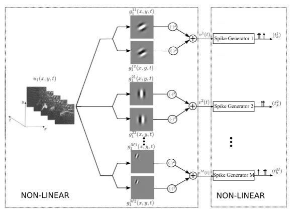
It is widely accepted that the early mammalian visual system employs a series of neural circuits to extract elementary visual features, such as edges and motion [1, 2]. Feature extraction capabilities of simple and complex cells arising in the primary visual cortex (V1) have been extensively investigated. Layer IV simple cells receive direct input from the Lateral Geniculate Nucleus [3]. Each simple cell consists of a linear receptive field cascaded with a highly nonlinear spike generator. Complex cells in layer II/III of V1 sum the output of a pool of simple cells having similar orienta-tion selectivity and spatial extent [4] and are thereby selective to oriented edges/lines over a spatially restricted region of the visual field [1]. Whereas simple cells respond maximally to a particular phase of the edge, complex cells are largely phase invariant [5,6]. Therefore, the receptive fields of complex cells cannot be simply mapped into excitatory and inhibitory regions [1]. Receptive fields of simple cells are often mod-eled as spatio-temporal linear filters with a spatial impulse response that resemble Gabor functions [7], whereas the receptive fields of complex cells are often modeled as sums of squared linear filters [8]. For simplicity, a quadrature pair of space-time Gabor filters has been employed in an energy model of complex cells [9–11]. Neural circuits comprising complex cells constitute a highly nonlinear circuit as illustrated in Fig.1.
Feedforward projections from V1 to other cortical areas mainly originate from layer II/III [12], suggesting that complex cells play a critical role in relaying visual information processed in V1 to higher brain areas. Whereas tuning properties of in-dividual complex cells have been characterized [13,14], the information about visual stimuli that an ensemble of complex cells can provide and how efficiently they can represent such information has yet to be elucidated.
Fig. 1 A neural circuit consisting of a population of complex cells
rigorous identification algorithms for identifying linear receptive fields of simple cells [17]. By modeling the nonlinear processing in complex cells as Volterra den-dritic stimulus processors (DSPs) [18,19], the representation of stimuli encoded by spike times generated by neural circuits with complex cells was also exhaustively an-alyzed. Functional identification of a complex cell DSP was possible again thanks to the demonstrated duality between decoding and functional identification. Although these theoretical methods exhibit deep structural properties, they have been shown to be tractable only for decoding and functional identification problems of small dimen-sions. In their current form, they are not tractable due to the ‘curse of dimensionality’ [20].
The nonlinear transformations taking place in the DSP of complex cells lead to loss of phase information. Previous work has empirically found that static images recovered from the magnitude response of Gabor wavelets are perceptually recog-nizable, albeit they exhibit significant errors in their pixel intensity values [21]. With this in mind, we formulate the reconstruction of stimuli encoded with complex cells as a phase retrieval problem [22] and, in search of tractable algorithms, utilize recent developments in optimization theory of low-rank matrices [22–24]. Applying such methods, we develop algorithms that are highly effective in decoding visual stimuli encoded by complex cells. As will be detailed in the next sections, the complex cells, as defined in this paper, have DSP kernels that are low-rank and include those shown in Fig.1as a particular case.
in [18], we show in this paper that these results remain valid under the assumption of sparsity, that is, for the case of low-rank DSP kernels. This significantly reduces the time of stimulus presentation that is needed in the identification process. The sparse duality result also enables us to evaluate the identified circuits in the input space. We achieve the latter by computing the mean square error or signal-to-noise ratio (SNR) of novel stimuli decoded using the identified circuits [17]. The sparse de-coding and functional identification algorithms presented here apply to circuits build around a wide range of neuron models including integrate-and-fire neurons with ran-dom thresholds and biophysically realistic conductance-based models with intrinsic noise.
This paper is organized as follows. In Sect.2, we first introduce the modeling of encoding of temporal stimuli with complex cells. We provide a detailed review of decoding of stimuli and the functional identification of complex cells and point out the current algorithmic limitations. In Sect.3, we provide sparse decoding algorithms that achieve high accuracy and are algorithmically tractable. We then explicate the dual relationship between sparse functional identification and decoding and provide examples for the identification of low-rank temporal DSP kernels of complex cells. In Sect.4, we extend sparse decoding methodology to spatio-temporal stimuli and functional identification of spatio-temporal complex cells. Using novel stimuli, we provide evaluation examples of the identification algorithms in the input space and compare them with other state-of-the-art methods. Finally, we conclude in Sect.5 and suggest how the approach advanced in this paper can be applied beyond complex cells.
2 Neural Circuits with Complex Cells: Encoding, Decoding, and
Functional Identification
In this section, we model the encoding of temporal stimuli by a neural circuit con-sisting of neurons akin to complex cells. We start by modeling the space of temporal stimuli in Sect.2.1. In Sect.2.2, the model of encoding is formally described. In Sect.2.3, we proceed to present a reconstruction algorithm for decoding temporal stimuli encoded by the neural circuit. A method for functional identification of neu-rons constituting the neural circuit is provided in Sect.2.4. The reconstruction algo-rithm and the functional identification algoalgo-rithm discussed in this section are based on [18].
2.1 Modeling Temporal Stimuli
We model the temporal varying stimuliu1=u1(t ),t∈D, as real-valued elements of
the space of trigonometric polynomials [15]. The choice of the space of the trigono-metric polynomials has, as we will see, substantial computational advantages.
Definition 1 The space of trigonometric polynomials H1 is the Hilbert space of
complex-valued functions
u1(t )=
Lt
lt=−Lt
over the domainD= [0, St], where
elt(t )=
1
√ St
exp
j ltΩt
Lt
t
,
andclt,lt= −Lt, . . . , Lt, are the coefficients ofu1inH1. HereΩtdenotes the
band-width, andLt is the order of the space. Stimuliu1∈H1are extended to be periodic
overRwith periodSt=2π Lt/Ωt.
We denote the dimension ofH1by dim(H1), and dim(H1)=2Lt+1.
Definition 2 The tensor product space H2=H1⊗H1 is the Hilbert space of
complex-valued functions
u2(t1;t2)=
Lt
lt1=−Lt
Lt
lt2=−Lt
dlt1lt2elt1(t1)·elt2(t2) (2)
over the domainD2= [0, St] × [0, St], wheredlt1lt2,lt1lt2 ∈D
2, are the coefficients
ofu2inH2.
Note that dim(H2)=dim(H1)2.
2.2 Encoding of Temporal Stimuli by a Population of Complex Cells
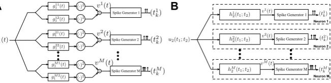
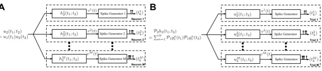
We consider a neural circuit consisting ofM neurons as shown in Fig.2A. For the
ith neuron, input stimulusu1(t )(u1∈H1) is first processed by two linear filters with
impulse responsesg1i1(t )andg1i2(t ), the outputs of which are individually squared and then summed together. These processing elements are integral part of the DSP of neuroni [18, 19]. The output of the DSP i, denoted by vi(t ), is then fed into the biological spike generator (BSG) of neuroni. The BSGiencodes the output of DSPiinto the spike train(tki)k∈Ii. HereIiis the spike train index set of neuroni. We
notice the similarity between the overall structure of neural circuits in Figs.2A and1. In what follows, we refer to the neurons in the neural circuit in Fig.2A as complex cells.
The output of the DSP of theith neuron in Fig.2A amounts to
vi(t )=
Dg i1
1(t−s1)u1(s1) ds1 2
+
Dg i2
1 (t−s2)u1(s2) ds2 2
(3)
for alli=1,2, . . . , M. With
hi2(t1;t2)=gi11(t1)g1i1(t2)+g1i2(t1)g1i2(t2), (4)
(3) can be rewritten as
vi(t )=
D2
Fig. 2 The encoding of temporal stimuli by a neural circuit modeling an ensemble of complex cells. (A) Theith neuron in the model processes the inputu1(t )by two parallel linear filters with impulse responsesgi11(t )andg1i2(t ), respectively, followed by squaring. The outputs are summed and then fed into a spike generator. (B) An equivalent representation of the encoding circuit in which the DSPs are represented as second-order Volterra kernels
wherehi2(t1;t2)is interpreted as a second-order Volterra kernel [25]. We assume that hi2(t1;t2)is real, bounded-input bounded-output (BIBO) stable, causal, and of finite
memory. The I/O of the neural circuit shown in Fig.2A can be equivalently outlined as in Fig.2B, in which each neuron processes the inputu1(t )nonlinearly by a
second-order kernelhi2(t1;t2)followed by a BSG.
Remark 1 Note that the BSG models the spike generation mechanism of the axon
hillock of a biological neuron, whereas the DSP is an equivalent model of processing of the stimuli by a sophisticated neural network that proceeds the spike generation. Therefore, stimulus processing and the spike generation mechanism are naturally sep-arated in the neuron model considered here.
For simplicity, we first formulate the spike generation mechanism of the encoder as an ideal integrate-and-fire (IAF) (point) neuron (see, e.g., [17]). The integration constant, bias, and threshold of the IAF neuroni=1,2, . . . , M are denoted byκi,
bi, andδi, respectively. The mapping of the input amplitude waveform vi(t ) into the time sequence(tki)k∈Ii is called the t-transform [15]. For theith neuron, the
t-transform is given by [15,16]
tki+1
tki
vi(t ) dt=κiδi−bitki+1−tki , k∈Ii. (6)
Lemma 1 The encoding of the temporal stimulusu1∈H1 into the spike train
se-quence(tki),k∈Ii,i=1,2, . . . , M, by a neural circuit with complex cells is given in
functional form by
Ti
ku2=qki, k∈Ii, i=1, . . . , M, (7) whereMis the total number of neurons,ni+1 is the number of spikes generated by neuroni, andTi
k :H2→Rare bounded linear functionals defined by
Ti ku2=
tki+1
tki
D2
hi2(t−s1;t−s2)u2(s1;s2) ds1ds2dt (8)
Proof Relationship (7) follows by replacing the functional form ofvi(t )given in (5)
in equation (6).
Remark 2 The functionu2(t1, t2)=u1(t1)·u1(t2)can be interpreted as a nonlinear map of the stimulusu1intou2defined in a higher-dimensional space. The operation
performed by the second-order Volterra kernel onu2in (8) is linear. Thus, (7) shows that the encoding of temporal stimuli can be viewed as generalized sampling [18].
The above formalism for encoding stimuli with complex cells can be extended in several ways. First, conductance-based BSGs, such as the Hodgkin–Huxley and Morris–Lecar neuron models, and Izhikevich point neuron models, can be employed [26–29]. The encoding can be similarly formulated as generalized sampling [16]. Second, to capture the stochastic nature of spiking neurons, intrinsic noise can be added into the BSG models. For example, an IAF neuron with random thresholds can be used [15,30]. It is also natural to consider intrinsic noise in the conductance-based BSGs [19]. For both models, it has been shown that the encoding of stimuli can be viewed as generalized sampling with noisy measurements [15,19], that is, the t-transform is of the form
Ti
ku2=qki +ε i
k, k∈I i, i=
1, . . . , M, (9)
whereTki are bounded linear functionals defined according to the neuron model of choice, andεki represents random noise in the measurements.
In what follows, we will mainly focus on encoding circuits consisting of complex cells whose spiking mechanism is modeled by a deterministic IAF neuron. The results obtained can be extended to the above two cases, and we will provide examples for both of these.
2.3 Decoding of Temporal Stimuli Encoded by a Population of Complex Cells
Assuming that the spike times(tki), k∈Ii,i=1,2, . . . , M, are known, by Lemma1 the neural circuit with complex cells encodes the stimulus via a set of linear function-als acting onu2(see equation (7)). Thus, the reconstruction ofu2can in principle be obtained by inverting the set of linear equations (7) [18].
Theorem 1 The coefficients ofu2∈H2in (2) satisfy the following system of linear
equations:
Ξd=q, whereΞ=Ξ1 T, . . . ,ΞM TT and q=q1 T, . . . ,qM TT
(10)
with[qi]k=qki,[d]lt1lt2 =dlt1lt2, and
Ξi
k;lt1lt2 = tki+1
tki
elt1+lt2(t ) dt
D2
This result can be obtained by plugging (2) into (7). We refer readers to Theorem 1 in [18] for a detailed proof.
We formulate the reconstruction ofu2as the following optimization problem:
ˆ
u2(t1;t2)=arg min
u2∈H2
M
i=1
k∈Ii
Ti ku2−qki
2
. (11)
Algorithm 1 The solution to (11) is given by
ˆ
u2(t1;t2)=
Lt
lt1=−Lt
Lt
lt2=−Lt ˆ
dlt1lt2elt1(t1)·elt2(t2), (12)
wheredˆ= [ ˆd−Lt,−Lt, . . . ,dˆ−Lt,Lt, . . . , . . . ,dˆLt,−Lt, . . . ,dˆLt,Lt]
T is obtained by
ˆ
d=Ξ†q (13)
with†denoting the pseudoinverse operator.
We note that a necessary condition for perfect recovery is that the total number of spikes exceeds dim(H1)(dim(H1)+1)/2+M[19]. Therefore, the complexity of the decoding algorithm is of order dim(H1)2.
Following [18,19], the decoding algorithm is called a Volterra time decoding ma-chine (Volterra TDM).
2.4 Functional Identification of DSPs of Complex Cells
In this section, we formulate the functional identification of a single complex cell in the neural circuit described in Fig. 2A. We perform M experimental trials. In trial i, i=1, . . . , M, we present a controlled stimulus ui1(t ) to the cell and ob-serve the spike times (tki)k∈Ii. We assume that the cell has a DSP of the form h2(t1;t2)=g11(t1)g11(t2)+g21(t1)g12(t2)and an integrate-and-fire BSG with
integra-tion constant, bias, and threshold denoted byκ, b, andδ, respectively. The objective is to functionally identifyh2from the knowledge ofui1and the observed spikes(tki)k∈Ii, i=1, . . . , M. This is a standard practice in neurophysiology for inferring the func-tional form of a component of a sensory system [1].
Definition 3 Lethp∈L1(Dp),p=1,2, whereL1denotes the space of
Lebesgue-integrable functions. The operatorP1:L1(D)→H1given by (P1h1)(t )=
Dh1
t K1
t;t dt (14)
is called the projection operator from L1(D) to H1. Similarly, the operator P2:
L1(D2)→H2given by
(P2h2)(t1;t2)=
D2
Note, that P1ui1 =u1i for ui1 ∈ H1. Moreover, for ui2(t1, t2)=u1i(t1)ui1(t2),
P2ui2=ui2.
Lemma 2 WithMtrials of stimuliui2(t1;t2)=u1i(t1)ui1(t2),i=1, . . . , M, presented
to a complex cell having DSPh2(t1, t2), we have
Li
k(P2h2)=qki, k∈I i, i=
1, . . . , M, (16)
where
Li
k(P2h2)= tki+1
tki
D2
ui2(t−s1;t−s2)(Ph2)(t−s1;t−s2) ds1ds2dt (17)
and
qki =κiδi−bitki+1−tki . (18)
Proof See Appendix1.
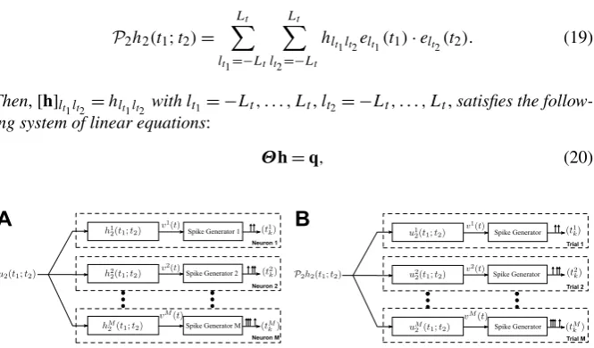
Remark 3 The similarity between equations (7) and (72) suggests that the identi-fication of a complex cell DSP by presenting multiple stimuli is dual to decoding a stimulus encoded by a population of complex cells. This duality is schematically shown in Fig.3.
Theorem 2 LetP2h2∈H2be of the form
P2h2(t1;t2)=
Lt
lt1=−Lt
Lt
lt2=−Lt
hlt1lt2elt1(t1)·elt2(t2). (19)
Then,[h]lt1lt2 =hlt1lt2 withlt1= −Lt, . . . , Lt,lt2= −Lt, . . . , Lt, satisfies the
follow-ing system of linear equations:
Θh=q, (20)
where Θ= [(Θ1)T, . . . , (ΘM)T]T and q= [(q1)T, . . . , (qM)T]T with [qi]k =qki and
Θik;l
t1lt2 = ti
k+1
tki
elt1+lt2(t ) dt
D2
ui2(s1;s2)e−lt1(s1)e−lt2(s2) ds1ds2. (21)
Thus, to identifyP2h2, we can follow the same methodology as in Algorithm1
and formulate the functional identification ofP2h2as
P2h2=arg min
P2h2∈H2
M
i=1
k∈Ii
Li
k(P2h2)−q i k
2
. (22)
For a detailed proof, we refer the reader to the proof of Theorem 1 in [18].
Algorithm 2 The solution to (22) is given by
P2h2(t1;t2)=
Lt
lt1=−Lt
Lt
lt2=−Lt ˆ
hlt1lt2elt1(t1)·elt2(t2), (23)
wherehˆ= [ ˆh−Lt,−Lt, . . . ,hˆ−Lt,Lt, . . . , . . . ,hˆLt,−Lt, . . . ,hˆLt,Lt]
T is obtained by
ˆ
h=Θ†q. (24)
The methodology described in Algorithm2to identify the nonlinear DSP is called the Volterra channel identification machine (Volterra CIM) [18,19].
Remark 4 Formulating the decoding and identification problems in the tensor product
spaceH2allows the identification of nonlinear processing by solving a set of linear
equations. However, due to the increased dimensionality, the algorithm requires for decodingO(dim(H1)2)measurements.
3 Low-Rank Decoding and Functional Identification
As shown in Sect.2.3, a reconstruction of the signalu2is in principle possible by
3.1 Low-Rank Decoding of Stimuli
3.1.1 Exploiting the Structure of Complex Cell Encoding
In Theorem1, we introduced a vector notation for the coefficients ofu2, d= [d−Lt,−Lt, . . . , d−Lt,Lt, . . . , . . . , dLt,−Lt, . . . , dLt,Lt]
T. (25)
We introduce here the matrix notation of the coefficients foru2∈H2:
D= ⎡ ⎢ ⎣
d−Lt,Lt . . . d−Lt,−Lt ..
. . .. ... dLt,Lt . . . dLt,−Lt
⎤ ⎥
⎦. (26)
We notice the following: (i) since u2 is assumed to be real, dlt1,lt2 =d−lt1,−lt2,
and (ii) sinceu2(t1;t2)=u1(t1)u1(t2)=u1(t2)u1(t1)=u2(t2;t1), we havedlt1,lt2 = dlt2,lt1. These properties imply that D is a Hermitian matrix. Moreover, we note that u2in (7) is the ‘outer’ product of the stimuliu1, that is,
D=ccH, (27)
where
c= [c−Lt, . . . , cLt]
T
(28)
are the coefficients of the basis functions ofu1. Therefore, D is a rank-1 Hermitian
positive semidefinite matrix. This property will be exploited in stimulus decoding (reconstruction).
Theorem 3 Encoding the stimulusu1∈H1with the neural circuit with complex cells
given in (6) into the spike train sequence(tki),k∈Ii,i=1,2, . . . , M, satisfies the set
of equations
TrΦikD =qki, k∈Ii, i=1, . . . , M, (29)
where Tr(·)is the trace operator, D is the rank-1 positive semidefinite Hermitian ma-trix D=ccH,qki =κiδi−bi(tki+1−tki)and(Φik),k∈Ii,i=1, . . . , M, are Hermitian
matrices with entries in the(lt2+Lt+1)th row and(lt1+Lt+1)th column given by
Φikl
t2,lt1=
ti k+1
tki
elt1−lt2(t ) dt
D2
hi2(s1;s2)e−lt1(s1)elt2(s2) ds1ds2. (30)
Proof Plugging in the general form ofu2 in (2) into (8), the left-hand side of (7) amounts to
Lt
lt1=−Lt
Lt
lt2=−Lt dlt1,−lt2
tki+1
tki
elt1−lt2(t ) dt
D2
It is easy to verify that this expression can be written as
Lt
lt1=−Lt
Lt
lt2=−Lt dlt1,−lt2
Φikl
t2,lt1 =Tr
ΦikD . (31)
Finally, we note that sincehi2,i=1, . . . , M, are assumed to be real valued, (Φik),
k∈Ii,i=1, . . . , M, are Hermitian.
Remark 5 We note that equation (29) in Theorem3and equation (10) in Theorem1 are the same. These equations represent the t-transform of a complex cell in (rank-1) matrix and vector form, respectively. The (rank-(rank-1) matrix representation is made possible by the equalityu2(t1;t2)=u1(t1)u1(t2).
3.1.2 Reconstruction Algorithms
Solving the systems of equations (29) and (10) requires at least dim(H1)(dim(H1)+
1)/2+M measurements. Consequently, practical solutions become quickly in-tractable. Fortunately, the encoded stimulus is of the formu2(t1;t2)=u1(t1)u2(t2).
This guarantees that D is a rank-1 matrix, and thus the reconstructed stimulus belongs to a small subset ofH2. Therefore, we can cast the problem of reconstructing
tem-poral stimuli encoded by neural circuits with complex cells as a feasibility problem, that is, finding all positive semidefinite Hermitian matrices that satisfy (29) and have rank 1. As we will demonstrate, the latter condition can be satisfied with substantially fewer measurements.
Recently, there is an increasing interest in low-rank optimizations such as matrix factorization, matrix completion, and rank minimization, both from a theoretical and from a practical standpoint [24,31,32]. For example, rank minimization has recently been applied to phase retrieval problems [22].
Our objective here is to find rank-1, positive semidefinite matrices that satisfy the t-transform (29). Since there always exists at least one rank-1 solution, this is equivalent to the following optimization problem [33]:
minimize Rank(D)
s.t. TrΦikD =qki, k∈Ii, i=1, . . . , M, D0.
(32)
The rank minimization problem in (32) is NP-hard. A well-known heuristic is to relax problem (32) to a trace minimization problem [32], that is, instead of solving (32), we reconstructu2using Algorithm3.
Algorithm 3 The reconstruction ofu2from the spike times generated by the neural circuit with complex cells is given by
ˆ
u2(t1;t2)=
Lt
lt1=−Lt
Lt
lt2=−Lt ˆ
where
ˆ D=
⎡ ⎢ ⎣ ˆ
d−Lt,Lt . . . dˆ−Lt,−Lt ..
. . .. ... ˆ
dLt,Lt . . . dˆLt,−Lt ⎤ ⎥
⎦ (34)
is the solution to the semidefinite programming (SDP) problem
minimize Tr(D)
s.t. TrΦikD =qki, k∈Ii, i=1, . . . , M, D0.
(35)
When the matrices(Φik),k∈Ii,i=1, . . . , M, satisfy the rank restricted isometry property [24], the trace norm relaxation converges to the true solution of (32), pro-vided that the number of measurements is of orderO(dim(H1)log(dim(H1)))[24].
These results suggest that stimuli encoded by complex cells can be decoded with a significantly lower number of measurements than that required by Algorithm1. To investigate this further, we applied the algorithm to decode a large number of stim-uli encoded by complex cells while varying the number of measurements (spikes) used by the decoding algorithm. The results show that the number of spikes required to faithfully represent a stimulus by a neural circuits consisting of complex cells is quasilinearly rather than quadratically proportional to the dimension of the stimulus space. These results are presented in the subsequent sections.
The matrix of weightsD obtained from the algorithm can be further decomposedˆ
to extract the signalu1(up to a sign) as follows.
(i) Perform the eigen-decomposition ofD. Denote the largest eigenvalue byˆ λand the corresponding eigenvector by v. If (35) does not exactly return a rank-1 matrix, then choose the largest eigenvalue and disregard the rest. Let w=√λv.
(ii) The reconstructed stimulusuˆ1is given by (up to a sign)
ˆ u1(t )=
Lt
lt=−Lt ˆ cltelt(t ),
where
ˆ c=
w·|[w]Lt+1|
[w]Lt+1 if[w]Lt+1=0,
w otherwise, (36)
withˆc= [ˆc−Lt, . . . ,cˆLt]
T, and[w]
Lt+1 is the(Lt +1)th entry of w, which
corre-sponds to the coefficientcˆ0.
IfD is rank 1, step (i) decomposesˆ D as an ‘outer’ product of a vector and itselfˆ
(see (27)). The resulting vector w differs from the actual coefficient vector of the stimulusu1by up to a complex-valued scaling factor. This factor is corrected in step (ii). Sinceu1is assumed to be real valued, the ‘DC’ component must be real valued. Therefore, we rotate w to remove any imaginary part. In practice, this also ensures
ˆ
Remark 6 Note that we can reconstructu1(t )up to a sign, since D=ccH and D= (−c)(−cH)are equally possible. For clarity, in all examples given in this paper, the sign of the recovered stimulus was matched to the original stimulus.
Remark 7 Note that (32) can be alternatively solved by replacing the objective with the log-det heuristic [32], that is,
minimize log det(D+λI)
s.t. TrΦikD =qki, k∈Ii, i=1, . . . , M, D0,
(37)
whereλ >0 is a small regularization constant. This optimization may further reduce the rank ofD when Algorithmˆ 3fails to progress to an exact rank-1 solution [32].
Remark 8 When intrinsic noise is present in the BSG, the encoding of stimuli can
be formulated as generalized sampling with noisy measurements. We modify (35) as follows:
minimize Tr(D)+λ M
i=1
k∈Ii
TrΦikD −qki 2
s.t. D0,
(38)
whereλcan be chosen based on the noise estimate. Here, the recovered D may no longer be rank-1. The largest rank-1 component is used for the reconstruction of stimuli.
Although the SDP in (35) provides an elegant way for relaxing the rank minimiza-tion problem, it is limited in practice by the need of large amounts of computer mem-ory for numerical calculations. The optimization problem (32) can also be solved using an alternating minimization scheme [34] as further outlined in Algorithm 4. The alternating minimization approach is more tractable when the dimension of the space is very large. Algorithm4uses an initialization step (step 1) that provides an initial iterate whose distance from D is bounded. It then alternately solves for the left and right singular vectors of the rank-1 matrix D while keeping the other one fixed (step 2). The resulting subproblems admit a straightforward least squares solution, which can be much more efficiently solved than the SDP in Algorithm3. Moreover, the algorithm is amenable to parallel computation using general purpose graphics processing units (GPGPUs). The latter property makes it even more attractive when the dimension of the stimulus space is large.
Algorithm 4
1. Initialize c1ˆ and c2ˆ to top left and right singular vectors, respectively, of
M i=1
k∈IiqkiΦiknormalized to
1
σ
M i=1
k∈Ii(qki)2, whereσis the top
singu-lar value ofMi=1k∈IiqkiΦik.
(a) solve forc1ˆ by fixingc2ˆ
ˆ
c1=arg min c1
M
i=1
k∈Ii
TrΦikc1cˆH2 −qki 2; (39)
(b) solve forˆc2by fixingc1ˆ
ˆ
c2=arg min c2
M
i=1
k∈Ii
TrΦikc1cˆ H2 −qki
2
(40)
untilMi=1∈Ii(Tr(Φikc1ˆ cˆH2 )−qki)2≤ , where >0 is the error tolerance level; 3. computeDˆ = ˆc1ˆcH2.
The matrixD approximates the coefficients ofˆ u2∈H2as in (33). We can
recon-structu1using the (appropriately scaled) top eigenvector of12(Dˆ + ˆDH). This can be
obtained directly fromc1ˆ andˆc2as follows. Let
k=ˆ
cH1c2ˆ − ˆcH2c1ˆ +
(cˆH1c2ˆ − ˆc2Hc1ˆ )2+4cˆH
1c1ˆˆ cH2c2ˆ
2cˆH
2c2ˆ
(41)
and
w=
1 2cˆ
H
2c1ˆ +kcˆH2ˆc2 ˆ c1+kc2ˆ
ˆc1+kc2 ˆ . (42)
The reconstructed stimulusu1ˆ is given by (up to a sign)
ˆ u1(t )=
Lt
lt=−Lt ˆ cltelt(t )
withc given by equation (ˆ 36).
We point out that we made the decoding manageable by exploiting the structure ofu2. Therefore, no constraint is imposed on the form thathi(t1;t2)takes, and the decoding algorithms can be applied to neural circuits with neurons whose DSPs take the form of any second-order Volterra kernel.
3.1.3 Example: Decoding Temporal Stimuli Encoded with a Population of Complex Cells
Here, the neural circuit we consider consists of 19 complex cells. The DSPs of the complex cells are of the form
where gi11(t ) and gi12(t ) are quadrature pairs of temporal Gabor filters, and i=
1, . . . ,19. The Gabor filters are constructed using a dyadic grid of dilations and trans-lations of the mother wavelets. The mother functions are given by
g11(t )=exp
−
t2
0.001
cos(40π t ) (44)
and
g12(t )=exp
−
t2
0.001
sin(40π t ). (45)
The ensemble of Gabor filters spans the frequency range of the input space. The BSG of the complex cells are point IAF neurons with biasbi =2 and integration constantκi=1,i=1, . . . , M. These two parameters are kept the same for all stimuli. Different threshold values are chosen for the IAF neurons to vary the total number of spikes, which can be used to evaluate how many measurements are required for perfectly reconstructing the input stimuli.
The domain of the input spaceH1isD= [0,1][sec], andLt=20,Ωt =20·2π
[rad/sec]. Thus, we have dim(H1)=41. The stimuli were generated by randomly choosing their basis coefficients from an i.i.d. Gaussian distribution.
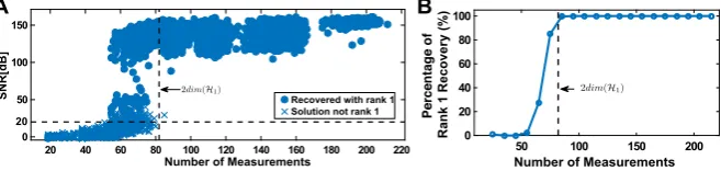
We tested the encoding and subsequent decoding of 6570 stimuli. The total num-ber of spikes produced for each stimulus ranged from 20 to 220. Reconstructions of the stimuli were performed using Algorithm3, and the SDPs were solved using SDPT3 [35].
We show the SNR of all reconstructions in the scatter plot of Fig.4A. Here solid dots represent exact rank 1 solutions (the largest eigenvalue is at least 100 times larger than the sum of the rest of the eigenvalues), and crosses indicate that the trace minimization found a higher rank solution that has a smaller trace. The percentage of exact rank 1 solutions is shown in Fig.4B. A relatively sharp transition from very low probability of recovery to very high rate of perfect reconstruction can be seen, similar to phase transition phenomena in other sparse recovery algorithms [36]. It can also be seen that the number of measurements that are needed for perfect recovery is substantially lower than the 861 spikes required by decoding based on Theorem1.
Fig. 4 Example of low-rank decoding. (A) Effect of number of measurements (spikes) on reconstruction
3.1.4 Example: IAF Spike Generators with Random Thresholds
Next, for the circuit presented in Sect.3.1.3, we assumed the IAF neurons to have random thresholds [15]. More specifically, during the interval[tki, tki+1), the threshold of theith neuron wasδki, whereδikare i.i.d. Gaussian random variables with meanδ
and varianceσ2. Since the thresholds are random, the spike times generated by the circuit are no longer deterministic.
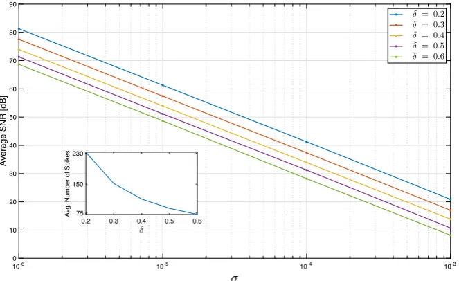
We chose five different values forδand four different values forσ. For each(δ, σ )
pair, we presented 50 stimuli to the circuit and subsequently decoded these by solving (38). We found that the SNR of the recovery degrades linearly with log(σ ). Figure5 depicts the average SNR of recovery as a function ofσfor variousδ. Note that a lower
δcorresponds to a higher number of spikes; the inset in the figure provides the average number of spikes produced by the circuit for eachδ. The results demonstrate that the low-rank decoding algorithm is stable to noise and applicable to non-deterministic encoding paradigms.
3.1.5 Example: Hodgkin–Huxley Neurons as Biophysical Spike Generators
Here, we evaluate the decoding of stimuli encoded by complex cells with BSGs mod-eled as Hodgkin–Huxley neurons. The space of the input stimuli and the structure of the DSPs of the neurons are the same as in Sects.3.1.3and3.1.4. However, as the Hodgkin–Huxley point neurons generate significantly more spikes than the IAF neu-rons considered in the previous examples, we only use here a total of five neuneu-rons.
Fig. 5 Robust reconstruction of temporal stimuli encoded by complex cells. The BSGs of the complex
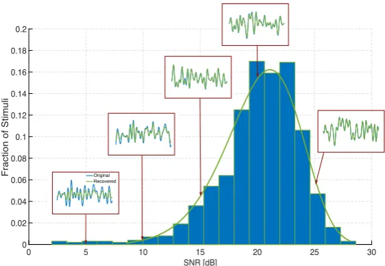
Fig. 6 Histogram of reconstruction SNRs of stimuli encoded by complex cells. The BSGs of the complex
cells are modeled as Hodgkin–Huxley point neurons. Insets show the original (blue) and recovered (green) stimuli for various SNR values
Again, the DSPs of these five neurons span the frequency range of the input space. We presented the circuit with 1000 stimuli and subsequently performed their sparse decoding. The average number of spikes generated by the circuit across all stimuli was 215. Figure6shows the histogram of the SNRs of the decoded stimuli, with the insets depicting the original and decoded waveforms of a few representative stimuli. These results demonstrate that the low-rank decoding framework presented in this section can also be applied to stimuli encoded with a wide range of spike generators, including the biophysically realistic conductance-based models.
3.1.6 Example: Hodgkin–Huxley Neurons with Stochastic Ion Channels
Finally, we again consider the same circuit as in Sect.3.1.5. However, intrinsic ion channel noise is added to the Hodgkin–Huxley point neurons. For a detailed mathe-matical treatment of Hodgkin–Huxley point neuron with stochastic ion channels, we refer the reader to [19]. Here, independent Brownian motion processes respectively drive each of the gating variables of the Hodgkin–Huxley neuron, that is,n (activa-tion of potassium channels),m(activation of sodium channels), andh(inactivation of sodium channels). The variances of the Brownian motion processes denoted by
σ12,σ22, andσ32 were respectively chosen to be 10σ1=σ2=σ3=σ. We presented
frame-Fig. 7 Robust reconstruction of stimuli encoded by complex cells with stochastic ion channels. The BSGs
are modeled as Hodgkin–Huxley point neurons with stochastic ion channels. For each noise levelσ, we set 10σ1=σ2=σ3=σwhereσi2,i=1,2,3, are the variances of the independent Brownian motion process driving the gating variablesn,m, andh, respectively. A largerσrepresents a higher intrinsic noise strength
work is robust to intrinsic noise in conductance-based spiking models up to a certain noise level.
3.2 Low-Rank Functional Identification of Complex Cells
3.2.1 Duality Between Low-Rank Functional Identification and Decoding
As discussed in Sect.2.4, the complexity of identification using Algorithm 2 can be prohibitively high. Often, a very large number of stimulus presentation trials are required to fully identify the DSP of biological neurons. To mitigate this, we consider exploiting the structure of the DSP of complex cells as motivated by the tractability of the low rank decoding algorithm.
We consider a single complex cell whose DSP is of the form
h2(t1;t2)=
N
n=1
g1n(t1)g1n(t2), (46)
whereg1n(t ),n=1, . . . , N, are impulse responses of linear filters, andNdim(H1). We note that a complex cell described in Fig.2A is a particular case of (46) withN=
2. A natural question here is whether, by assuming such a structure, the functional identification of complex cell DSPs is tractable.
Remark 9 It is well known that a second-order Volterra kernel has infinitely many
equivalent forms but has a unique symmetric form [25].
dual to decoding of low-rank stimuli, then it is straightforward to provide tractable algorithms for identifyingh2(t1;t2)of the form (46).
Since P1g1n(t )∈ H1, n=1, . . . , N, there is a set of coefficients (glnt), lt =
−Lt, . . . , Lt,n=1,2, . . . , N, such that
P1gn1(t )=
Lt
lt=−Lt gln
telt(t ). (47)
In what follows, we denote coefficients in vector form as
gn=g−nL t, . . . , g
n Lt
T
. (48)
Similarly, we denote the coefficients ofP1h2(t1;t2)in (19) in matrix form as
H= ⎡ ⎢ ⎣
h−Lt,Lt . . . h−Lt,−Lt ..
. . .. ... hLt,Lt . . . hLt,−Lt
⎤ ⎥
⎦. (49)
Then
H=
N
n=1
gngn H, (50)
and thus H is a Hermitian positive semidefinite matrix with rank at mostN.
Theorem 4 By presentingMtrials of stimuliui2(t1;t2)=ui1(t1)ui1(t2), i=1, . . . , M,
to a complex cell its coefficients satisfy the set of equations
TrΨikH =qki, k∈Ii, i=1, . . . , M, (51)
whereni+1, i=1, . . . , M, is the number of spikes generated by the complex cell in trial i, H is a Hermitian positive semidefinite matrix with rank(H)≤N given by H=Nn=1gn(gn)H with gn= [g−nL
t, . . . , g
n Lt]
T,(Ψi k), k∈I
i, i=1, . . . , M, are Hermitian matrices with entry at the(lt2+Lt+1)th row and(lt1+Lt+1)th column
given by
Ψik
lt2;lt1 =
tki+1
ti k
elt1−lt2(t ) dt
D2
ui2(s1;s2)e−lt1(s1)elt2(s2) ds1ds2. (52)
Proof From Lemma2we have
Li
k(P2h2)=q i
k, k∈I
i, i=1, . . . , M, (53)
where
Li
k(P2h2)=
ti k+1
tki
D2
ui2(t−s1;t−s2)(P2h2)(s1;s2) ds1ds2dt. (54)
Fig. 8 Duality between low-rank decoding and low-rank functional identification. Duality between
low-rank decoding of a stimulus encoded by a population of complex cells and low-rank functional iden-tification of complex cells. (A) The low-rank decoding algorithm assumes that the encoded stimulus can be written asu2(t1;t2)=u1(t1)u1(t2). (B) Functional identification of a complex cell assumes that the
structure of the DSP is low rank, that is,P2h2(t1;t2)=Nn=1P1gn1(t1)P1gn1(t2)
Remark 10 As in Sect.3.2, we note that the similarity in (51) and (29) indicates the duality between low-rank functional identification of complex cells and low-rank de-coding of stimuli encoded by a population of complex cells. The duality is illustrated in Fig.8.
3.2.2 Functional Identification Algorithms
To functionally identify the complex cell DSP, we again employ a rank minimization problem
minimize Rank(H)
s.t. TrΨikH =qki, k∈Ii, i=1, . . . , M, H0.
(55)
We relax the problem to a trace minimization problem similarly to the approach in the low-rank reconstruction algorithm. Here, the optimal solution will have rankN, however. Algorithm5is considered for low-rank functional identification of complex cells.
Algorithm 5 The functional identification of complex cell DSP from the spike times
generated by the neuron inMstimulus trials is given by
P2h2(t1;t2)=
Lt
lt1=−Lt
Lt
lt2=−Lt ˆ
hlt1lt2elt1(t1)·elt2(t2), (56)
where
ˆ H=
⎡ ⎢ ⎣ ˆ
h−Lt,Lt . . . hˆ−Lt,−Lt ..
. . .. ... ˆ
hLt,Lt . . . hˆLt,−Lt ⎤ ⎥
is the solution to the SDP problem
minimize Tr(H)
s.t. TrΨikH =qki, k∈Ii, i=1, . . . , M, H0.
(58)
Based on the results for decoding using Algorithm3and provided thath2is of the form (46), we intuitively inferred that the number of measurements for the perfect identification ofP2h2is much smaller thanO(dim(H1)2). We demonstrate that this
is the case for a large number of identification examples in the subsequent sections. This suggests that even if the dimension of the input space becomes large, the functional identification of the DSP of complex cells is still tractable. This result has critical implication for performing neurobiological experiments to functionally identify complex cells. First, it suggests that a much smaller number of stimulus trials is needed for perfect identification. Second, the total number of spikes/measurements that needs to be recorded can be significantly reduced. Both mean that the duration of experiment can be shortened.
Remark 11 Note that only the projection of the DSPh2onto the space of input stimuli can be identified.
Remark 12 We can use the largestNeigenvalues and their respective eigenvectors of
ˆ
H to obtain the projection of individual linear filter componentsP1g1n,n=1, . . . , N.
However, these components may not directly correspond toP1g1n,n=1, . . . , N, in
that the original projections may not be ‘orthogonal’, whereas the eigenvalue decom-position imposes orthogonality.
As in Algorithm4, when applied for solving the decoding problem, the rank min-imization problem above can be solved using alternating minmin-imization, as further de-scribed in Algorithm6. Here, we solve for the topN left and right singular vectors of
H alternately, whereNis the rank of the second-order Volterra DSP. We note that the initialization step is akin to running an algorithm very similar to the spike-triggered covariance (STC) algorithm widely used in neuroscience [37–41]. The subsequent steps then improve upon this initial estimate.
Algorithm 6
1. Initialize H1ˆ and H2ˆ to top N left and right singular vectors, respectively, of
M i=1
ni
k=1qkiΨ i
k with the nth singular vector normalized to
1
N ×
1
σn M
i=1 ni
k=1(q
i
k)2, whereσnis the topnth singular value of
M i=1
ni
k=1q
i k×
Ψik.
2. Solve the following two minimization problems: (a) solve forH1ˆ by fixingH2ˆ
ˆ
H1= arg min
H1∈Cdim(H1)×N
M
i=1
k∈Ii
(b) solve forH2ˆ by fixingH1ˆ
ˆ
H2= arg min
H2∈Cdim(H1)×N
M
i=1
k∈Ii
TrΨikH1Hˆ H2 −qki
2
(60)
until Mi=1∈Ii(Tr(ΨikH1ˆ HˆH2)−qki)2≤ , where >0 is the error tolerance
level;
3. computeHˆ =12(H1ˆ HˆH
2 + ˆH2HˆH1).
3.2.3 Example: Identification of Complex Cell DSPs from Spike Times
In this example, we consider identifying a single complex cell having the following Volterra DSP:
h2(t1, t2)=g11(t1)g11(t1)+g12(t1)g21(t2), (61)
where
g11(t )=50 exp
−(t−0.3)2
0.002
cos(40π t ), (62)
g12(t )=50 exp
−(t−0.3)2
0.002
sin(40π t ). (63)
In repeated trials, we presented to the complex cell 1-second long stimuli cho-sen from the input space. The domain of the input spaceH11isD= [0,1](sec) and
Lt=20,Ωt=20·2π(rad/sec), and thus dim(H11)=41. The stimuli were generated
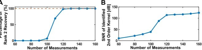
by independently choosing their basis coefficients from the same Gaussian distribu-tion. We presented a total of 16,600 different stimuli in the repeated trials. We then randomly selected between 30–80 trial subsets such that the total number of spikes in each subset was between 60 and 160. We performed the identification process on each subset using Algorithm5. The optimization problem was solved using SDPT3. For each instantiation of the identification algorithm, we recorded whether the optimization process resulted in a rank-2 solution and also the SNR of the identified DSP with respect to the original one. For the purpose of demonstration, we binned these results based on number of spikes used into bins of width 10. The percentage of rank-2 solutions is shown in Fig.9A as a function of number of measurements. The mean SNR is shown in Fig.9B.
It can be seen from Fig. 9B that the identification algorithm presented here is able to recover the underlying DSP with exceptional accuracy using a reasonable and tractable number of measurements.
3.3 Evaluation of Functional Identification of a Neural Circuit of Complex Cells by Decoding
Fig. 9 Example of low-rank functional identification. (A) Percentage of successful rank-2 recovery in
identification. (B) Mean SNR of identified second-order DSP kernel
that the proposed sparse functional identification algorithm enables the identification of complex cells with a tractable number of measurements. Together, the two algo-rithms afford us tractable functional identification of an entire neural circuit of com-plex cells that is capable of fully representing stimuli information, in that (i) the size of the neural circuit is tractable and (ii) the requirement for functional identification is tractable.
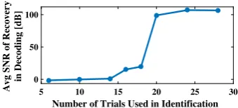
Decoding of visual stimuli by identified linear filters has previously been consid-ered in [42]. In [17], it was shown that the evaluation of functional identification of an entire neural circuit can be more intuitively performed in the input space by decoding the stimuli with identified circuit parameters. Here, we extend the previous results and apply such evaluation procedure on the sparse decoding and sparse functional identi-fication algorithms. The procedure is described as follows. First, each complex cell is functionally identified using Algorithm5or Algorithm6. Second, novel stimuli are presented to the neural circuit. Third, the spike trains observed are used to reconstruct the encoded novel stimuli by the sparse decoding algorithm, assuming that the circuit parameters take the identified values. Finally, SNR of the reconstruction can be ob-tained. A high SNR indicates a well-identified circuit, whereas a low number implies that the functional identification of the neural circuit is not of good quality. The latter can be caused by a lack of number of measurements used in functional identification or by a lack of complex cells in the neural circuit.
Fig. 10 Evaluating
identification quality in the input space. Identification quality was evaluated by plotting the average SNR of reconstruction of novel stimuli assumed to be encoded with the identified DSPs
4 Low-Rank Decoding and Functional Identification of Complex Cells
with Spatio-Temporal Stimuli
The framework introduced in Sect. 3 can be extended to the sparse decoding of spatio-temporal stimuli and the sparse identification of spatio-temporal DSPs of com-plex cells. Details of the extension to the spatio-temporal case are provided in Ap-pendixes2–4. In what follows, we present spatio-temporal examples of sparse decod-ing and identification.
4.1 Low-Rank Decoding of Spatio-Temporal Visual Stimuli
The stimuliu1considered here havepspatial dimensions and a single temporal di-mension, that is,u1=u1(x1, x2, . . . , xp, t ). For simplicity of notation, we use a
com-pact vector notation and denote the spatial variables as x=(x1, x2, . . . , xp). When
p=2,u1is the usual 2D visual stimulus. The definition of the space of input stimuli is provided in Appendix2.
The encoding of spatiotemporal stimuli by a population of complex cells and the sparse decoding of spatiotemporal stimuli are formally described in Appendix3. Note that the output of the DSP of each neuroni=1,2, . . . , M, can be expressed as
vi(t )=
D2
hi2(x1, t−s1;x2, t−s2)u1(x1, s1)u1(x2, s2)dx1dx2ds1ds2, (64) where
h2i(x1, t1;x2, t2)=g1i1(x1, t1)g1i1(x2, t2)+gi12(x1, t1)g1i2(x2, t2) (65)
has low-rank [18].
In this section, we provide examples that demonstrate the tractability of sparse de-coding of spatio-temporal stimuli encoded with complex cells using a small number of spikes.
4.1.1 Example: Decoding of 2D Spatio-Temporal Stimuli
We first present an example in which x is one-dimensional, that is, x=x1. In this example, our main focus is to illustrate how the number of spikes affects the recon-struction of stimuli encoded by complex cells.
The neural circuit we consider here consists of 62 direction selective complex cells. The low-rank DSPs of the complex cells are of the form
whereg1i1(x, t )andg1i2(x, t ) are quadrature pairs of spatio-temporal Gabor filters, andi=1, . . . , M. The Gabor filters are constructed from dilations and translations of the mother wavelets on a dyadic grid, where the mother functions are expressed as
g11(x, t )=exp
−
x12
8 +
t2
0.001
cos(1.5x1+20π t ) (67)
and
g21(x, t )=exp
−
x12
8 +
t2
0.001
sin(1.5x1+20π t ). (68)
The BSG of the complex cells are IAF neurons with bias bi =10 and integration constantκ =1 for i=1, . . . , M. These two parameters are kept the same for all stimuli. Different threshold values are chosen for the IAF neurons to vary the total number of spikes in a larger range to evaluate how many measurements are required for a perfect reconstruction of input stimuli.
The domain of the input spaceH11 isD= [0,32] × [0,0.4]([a.u.] and [sec], re-spectively) andLx1 =6, Lt =4, Ωx1 =0.1875·2π, Ωt =10·2π [rad/sec]. Thus, dim(H11)=117. Stimuli were randomly generated by choosing the basis coefficients to be i.i.d. Gaussian random variables.
We tested the encoding of 1416 stimuli. Each time, a different number of spikes was generated. The reconstruction of stimuli was performed in MATLAB using the extended Algorithm3, and the SDPs were solved using SDPT3 [35].
The SNR of all reconstructions is depicted in the scatter plot of Fig.11A. Here solid dots represent exact rank 1 solutions (largest eigenvalue is at least 100 times larger than the sum of the rest of the eigenvalues), and crosses indicate that the trace minimization found a higher rank solution with a smaller trace. The percentage of exact rank 1 solutions is shown in Fig.11B. Similar to phase transition phenom-ena in other sparse recovery algorithms [36], a relatively sharp transition (around 50 spikes) from very low probability of recovery to very high probability of perfect re-construction can be seen. It can also be seen that the number of measurements that are needed for perfect recovery is substantially lower than the 6965 spikes required by Algorithm1.
Fig. 11 Example of low-rank decoding of spatio-temporal stimuli. (A) Effect of number of measurements
4.1.2 Example: Decoding of 3D Spatio-Temporal Stimuli
Next, we present two examples of decoding of spatio-temporal visual stimuli encoded by a population of complex cells. Here, x=(x1, x2)and the Volterra DSPs of the complex cells are of the form
hi2(x1, t1;x2, t2)=gi11(x1, t1)g1i1(x2, t2)+g1i2(x1, t1)g1i2(x2, t2), (69) whereg1i1(x, t )andgi12(x, t )are, for simplicity, quadrature pairs of spatial-only Ga-bor filters, andi=1, . . . , M. The Gabor filters are constructed using a dyadic grid of dilations, translations, and rotations of the following pair of mother wavelets [15]:
g11(x, t )=exp
−1
8
4x12+2x22 cos(2.5x1) (70) and
g12(x, t )=exp
−1
8
4x12+2x22 sin(2.5x1). (71)
The ensemble of Gabor filters forms a frame in the spatial domain of the input space [43].
For the first example, a 0.4-second-long synthetically generated video sequence is encoded by the neural circuit. The order of the input space was chosen to be
Lx1 =Lx2 =3, Lt =4. Thus, the dimension of the input space is 441. The input stimulus was created by choosing its basis coefficients to be i.i.d. Gaussian random variables. The stimulus was encoded by a neural circuit consisting of 318 complex cells. A total of 1374 spikes were generated by the encoding circuit. The stimulus was decoded using the extended Algorithm3. As shown in Fig. 12, the video sequence can be perfectly reconstructed with a fairly small number of spikes (A snapshot of the video is shown; see also Supplementary Video S1 for full video). The SNR of the re-constructed video was 92.8 [dB], thereby reaching almost perfect reconstruction with machine precision. Note that without the reconstruction algorithm employed here, 97,461 measurements would be required from at least 5733 complex cells to achieve perfect reconstruction.
Fig. 12 Example of reconstruction of synthesized visual stimuli. A synthetically generated visual stimulus
We then performed encoding and subsequent reconstructions of 2-second long nat-ural video sequences that had a resolution of 72×128 pixels. The videos had temporal bandwidth of 10 [Hz] and spatial bandwidth of 0.375 cycles per pixel. Additionally, the spatial bandwidth was restricted to a circular area to make it isotropically ban-dlimited. The videos were encoded by a neural circuit consisting of 21,776 complex cells, whose DSPs were modeled as spatial-only quadrature pair of Gabor filters. The Gabor filters formed a frame in the spatial dimension of the space.
The decoding was performed using six NVIDIA P100 GPUs on a single computer node. Despite of their computational power, the amount of memory required by the algorithm for decoding the whole video sequence exceeded the memory capacity of the six GPUs. Therefore, the reconstruction of the entire video was performed by decoding 0.2-second-long segments of the video independently and then stitching them together [16]. The overlap between consecutive segments was 0.1 second. We chose the order of the space to beLx1 =27, Lx2 =48, Lt =3, and the bandwidth of the space to beΩx1=Ωx2 =0.75π [rads/pixel] andΩt =20π [rads/s]. We also restricted the spectral lines in the spatial dimension to be inside a circular area instead of a square area as defined in (73), that is, we considered onlylx1andlx2that are in the set{(lx1, lx2)|l
2
x1L
2
x2+l
2
x2L
2
x1≤L
2
x1L
2
x2}. This allowed the bandwidth of the stimuli to be covered with minimal number of spectral lines [16]. Note that, by the construction of input space, the decoded video must be periodic in time. However, an arbitrary 0.2-second video may not be periodic. Therefore, we chose the decoding space to have a temporal period of 0.3 seconds and retained only the middle 0.2 seconds of the reconstructed segments. The total dimension of the decoding space was 28,413. The extended Algorithm4was used in decoding.
For the example depicted in Fig.13A, a total of 980,730 spikes were generated by the neural circuit. About 76,000 to 86,500 measurements were used in reconstructing the video in each time segment. This is approximately 2.67 to 3.04 times of the di-mension of the space. In contrast, a total of 403,663,491 measurements would have been required by Algorithm1to reconstruct the same video. In Fig.13A, snapshots of the original video sequence, the reconstructed video sequence and the error are shown (see also Supplementary Video S2) The SNR of the reconstructed video was 48.85 [dB] (the first and last 20 milliseconds were removed from the SNR calculation due to boundary conditions).
Additional examples of reconstructed natural video encoded by the same neural circuit are shown in Fig.13B–E (see also Supplementary Video S3–S6).
4.2 Low-Rank Functional Identification of Spatio-Temporal Complex Cells
The low-rank functional identification described in Sect.3.2can be extended to iden-tify DSPs of spatio-temporal complex cells. The functional identification for the spatio-temporal case is formally described in Appendix4.
Fig. 13 Examples of reconstruction of natural visual stimuli. Snapshots of the original videos encoded
by a neural circuit with complex cells are shown on the left. The reconstructions from the spike times are shown in the middle and the error on the right. Note that the color bar indicating the magnitude of the error was set to 10% of the input range. SNR: (A) 48.85 [dB]. (B) 46.92 [dB]. (C) 48.61 [dB]. (D) 50.76 [dB].
(E) 48.11 [dB]. (See also Supplementary Videos S2–S6)
4.2.1 Example: Low-Rank Functional Identification of Complex Cell DSP from Spike Times in Response to Spatio-Temporal Stimuli
In this example, we first consider identifying the DSP of a single complex cell in the neural circuit used in Sect.4.1.1. As a reminder, the neural circuit used in the example in Sect.4.1.1encodes spatio-temporal stimuli of the formu1(x1, t ).
We presented to the population of M complex cells 0.4-second stimuli, where