IJSRSET1848148 | Received : 15 June 2018 | Accepted : 26 June 2018 | May-June-2018 [(4) 8 : 640-645]
640
An Efficient Algorithm for Real-Time Object Detection in Images
Md. Samiul Islam, Samia Sultana
Stamford University Bangladesh, Dhaka, Bangladesh ABSTRACT
In this paper we have proposed an algorithm for object detection in various situations. Nowadays object detection and recognition has entered in every sphere of life in one or the other form. Applications of object detection are video surveillance, anti-theft system using cameras, face-recognition, biometric verification etc. Research are going on how to improve the performance in term of space and time complexity, how to deal with adverse conditions like improper lightning conditions, scene clutter, occlusion etc. and to reduce false positive rate etc. In this paper we have explained how to deal with the any situation while acquiring the images so that it can be used for better scene interpretation. Results have been generated using flash of light and dark region present in the image as some of the adverse situations. Here we have trained the system to detect the object using our algorithm. The algorithm is simple and very useful as it reduces the false positive rate as compared to contemporary algorithms and increases the efficiency of applications like video surveillance and scene interpretation etc.
Keywords: Object Detection, Image Classification, Image Recognition, Histogram of Oriented Gradients, Support Vector Machine.
I.
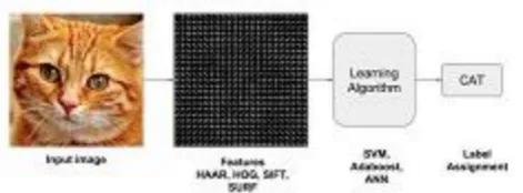
INTRODUCTIONAn image recognition algorithm takes an image (or a patch of an image) as input and outputs what the image contains. In other words, the output is a class label (e.g. “cat”, “dog”, “table” etc.). How does an image recognition algorithm know the contents of an image? Well, we have to train the algorithm to learn the differences between different classes. If we want to find cats in images, we need to train an image recognition algorithm with thousands of images of cats and thousands of images of backgrounds that do not contain cats. Needless to say, this algorithm can only understand objects / classes it has learned.
To simplify things, we will focus only on two-class (binary) classifiers. One may think that this is a very limiting assumption, but many popular object detectors (e.g. face detector and pedestrian detector)
have a binary classifier under the hood. E.g. inside a face detector is an image classifier that says whether a patch of an image is a face or background.
The following diagram illustrates the steps involved in a traditional image classifier.
Figure 1: Object (cat) detection using traditional image processing
Deep Learning based algorithms bypass the feature extraction step completely.
II.
METHODS AND MATERIALA. Preprocessing
Often an input image is pre-processed to normalize contrast and brightness effects. A very common preprocessing step is to subtract the mean of image intensities and divide by the standard deviation. Sometimes, gamma correction produces slightly better results. While dealing with color images, a color space transformation (e.g. RGB to LAB color space) may help get better results.
We evaluated several input pixel representations including grayscale, RGB and LAB color spaces optionally with power law (gamma) equalization. These normalizations have only a modest effect on performance, perhaps because the subsequent descriptor normalization achieves similar results. We do use colour information when available. RGB and LAB colour spaces give comparable results, but restricting to grayscale reduces performance by 1.5% at 10−4 FPPW. Square root gamma compression of each colour channel improves performance at low FPPW (by 1% at 10−4 FPPW) but log compression is too strong and worsens it by 2% at 10−4 FPPW.”
As part of pre-processing, an input image or patch of an image is also cropped and resized to a fixed size. This is essential because the next step, feature extraction, is performed on a fixed sized image.
B. Feature Extraction
The input image has too much extra information that is not necessary for classification. Therefore, the first step in image classification is to simplify the image by extracting the important information contained in the image and leaving out the rest. For example, if we want to find shirt and coat buttons in images, we will notice a significant variation in RGB pixel values.
However, by running an edge detector on an image we can simplify the image. We can still easily discern the circular shape of the buttons in these edge images and so we can conclude that edge detection retains the essential information while throwing away non-essential information. The step is called feature extraction. In traditional computer vision approaches designing these features are crucial to the performance of the algorithm. Turns out we can do much better than simple edge detection and find features that are much more reliable. In our example of shirt and coat buttons, a good feature detector will not only capture the circular shape of the buttons but also information about how buttons are different from other circular objects like car tires.
Some well-known features used in computer vision are Haar-likefeatures introduced by Viola and Jones, Histogram of Oriented Gradients ( HOG ), Scale-Invariant Feature Transform ( SIFT ), Speeded Up Robust Feature ( SURF ) etc.
As a concrete example, please look at feature extraction using Histogram of Oriented Gradients ( HOG ).
Histogram of Oriented Gradients (HOG)
A feature extraction algorithm converts an image of fixed size to a feature vector of fixed size. In the case of pedestrian detection, the HOG feature descriptor is calculated for a 64×128 patch of an image and it returns a vector of size 3780. Notice that the original dimension of this image patch was 64 x 128 x 3 = 24,576 which is reduced to 3780 by the HOG descriptor.
Step 1: Gradient calculation: Calculate the x and the y gradient images, and , from the original image. This can be done by filtering the original image with the following kernels.
Using the gradient images and , we can calculate the magnitude and orientation of the gradient using the following equations.
The calcuated gradients are unsigned and therefore is in the range 0 to 180 degrees.
Step 2: Cells: Divide the image into 8×8 cells.
Step 3: Calculate histogram of gradients in these 8×8 cells: At each pixel in an 8×8 cell we know the gradient (magnitude and direction), and therefore we have 64 magnitudes and 64 directions—i.e. 128 numbers. Histogram of these gradients will provide a more useful and compact representation. We will next convert these 128 numbers into a 9-bin histogram (i.e. 9 numbers). The bins of the histogram correspond to gradients directions 0, 20, 40 … 160 degrees. Every pixel votes for either one or two bins in the histogram. If the direction of the gradient at a pixel is exactly 0, 20, 40 … or 160 degrees, a vote equal to the magnitude of the gradient is cast by the pixel into the bin. A pixel where the direction of the gradient is not exactly 0, 20, 40 … 160 degrees splits its vote among the two nearest bins based on the distance from the bin. E.g. A pixel where the magnitude of the gradient is 2 and the angle is 20
degrees will vote for the second bin with value 2. On the other hand, a pixel with gradient 2 and angle 30 will vote 1 for both the second bin (corresponding to angle 20 ) and the third bin ( corresponding to angle 40 ).
Step 4: Block normalization : The histogram calculated in the previous step is not very robust to lighting changes. Multiplying image intensities by a constant factor scales the histogram bin values as well. To counter these effects we can normalize the histogram — i.e. think of the histogram as a vector of 9 elements and divide each element by the magnitude of this vector. In the original HOG paper, this normalization is not done over the 8×8 cell that produced the histogram, but over 16×16 blocks. The idea is the same, but now instead of a 9 element vector we have a 36 element vector.
Step 5: Feature Vector: In the previous steps we figured out how to calculate histogram over an 8×8 cell and then normalize it over a 16×16 block. To calculate the final feature vector for the entire image, the 16×16 block is moved in steps of 8 ( i.e. 50% overlap with the previous block ) and the 36 numbers (corresponding to 4 histograms in a 16×16 block ) calculated at each step are concatenated to produce the final feature vector. What is the length of the final vector?
The input image is 64×128 pixels in size, and we are moving 8 pixels at a time. Therefore, we can make 7 steps in the horizontal direction and 15 steps in the vertical direction which adds up to 7 x 15 = 105 steps. At each step we calculated 36 numbers, which makes the length of the final vector 105 x 36 = 3780.
C. Learning Algorithm for Classification
Before a classification algorithm can do its magic, we need to train it by showing thousands of examples of cats and backgrounds. Different learning algorithms learn differently, but the general principle is that learning algorithms treat feature vectors as points in higher dimensional space, and try to find planes / surfaces that partition the higher dimensional space in such a way that all examples belonging to the same class are on one side of the plane / surface.
To simplify things, let us look at one learning algorithm called Support Vector Machines (SVM) in some detail.
Support Vector Machine (SVM) is one of the most popular supervised binary classification algorithm. Although the ideas used in SVM have been around since 1963, the current version was proposed in 1995 by Cortes and Vapnik.
In the previous step, we learned that the HOG descriptor of an image is a feature vector of length 3780. We can think of this vector as a point in a 3780-dimensional space. Visualizing higher 3780-dimensional space is impossible, so let us simplify things a bit and imagine the feature vector was just two dimensional.
Figure 2: Classifying image points using SVM
In our simplified world, we now have 2D points representing the two classes (e.g. cats and
background). In the image above, the two classes are represented by two different kinds of dots. All black dots belong to one class and the white dots belong to the other class. During training, we provide the algorithm with many examples from the two classes. In other words, we tell the algorithm the coordinates of the 2D dots and also whether the dot is black or white.
Different learning algorithms figure out how to separate these two classes in different ways. Linear SVM tries to find the best line that separates the two classes. In the figure above, H1, H2, and H3 are three lines in this 2D space. H1 does not separate the two classes and is therefore not a good classifier. H2 and H3 both separate the two classes, but intuitively it feels like H3 is a better classifier than H2 because H3 appears to separate the two classes more cleanly. Why? Because H2 is too close to some of the black and white dots. On the other hand, H3 is chosen such that it is at a maximum distance from members of the two classes.
Given the 2D features in the above figure, SVM will find the line H3 for us. If we get a new 2D feature vector corresponding to an image the algorithm has never seen before, we can simply test which side of the line the point lies and assign it the appropriate class label. If our feature vectors are in 3D, SVM will find the appropriate plane that maximally separates the two classes. If our feature vector is in a 3780-dimensional space, SVM will find the appropriate hyperplane.
Optimizing SVM
training examples are classified properly. This tradeoff is controlled by a parameter called C. When the value of C is small, a large margin hyperplane is chosen at the expense of a greater number of misclassifications. Conversely, when C is large, a smaller margin hyperplane is chosen that tries to classify many more examples correctly.
III.
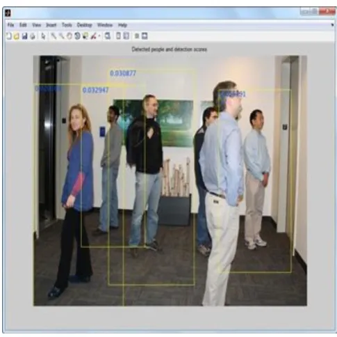
RESULTS AND DISCUSSIONThe results of our proposed algorithm are shown in Figure 3 and Figure 4.
It can be seen from the Figure 3 and Figure 4 that the proposed algorithm can accurately detect objects such as humans and car. In addition, the moving car is also difficult to detect in the detection task. But the moving car can be detected by the proposed algorithm. In summary, the proposed algorithm can achieve better results of these samples and locate the objects reasonably.
Figure 3: Human detection using pretrained SVM with HOG features.
Figure 4: Moving cars detection using SVM classifier
IV.
CONCLUSIONOn the basis of summarizing the limitations of the existing algorithm for the object detection, this paper presents object detection based on deep learning of small samples. The proposed algorithm contains modules as: preprocessing, feature extraction and support vector machine, which can realize object detection of a scene. Experimental results show the proposed method is significantly better than the existing techniques in terms of both subjective and objective. In the future work, we will combine object detection with attitude estimation to make the object detector better used in the service robotics.