An Approximate Solution of the two dimensional Unsteady Flow due to Normally Expanding or Contracting Parallel Plates

(1)

ISSN (online): 2349-784X

An Approximate Solution of the Two Dimensional

Unsteady Flow due to Normally Expanding or

Contracting Parallel Plates

Vishal V. Patel Jigisha U. Pandya

Assistant Professor Assistant Professor

Department of Mathematics Department of Mathematics

Shankersinh Vaghela Bapu Institute of Technology, Gandhinagar, Gujarat

Sarvajanik college of Engineering & Technology, Surat, Gujarat

Abstract

The flow of a viscous incompressible fluid between two parallel plates due to the normal motion of the plates for the two-dimensional flow is investigated. The governing nonlinear equations and their associated boundary conditions are transformed into linear differential equation using quasilinearization technique. The solution of the problem is obtained by Quintic spline collocation method. Graphical results are presented to investigate the influence of the squeeze number on the velocity, skin friction, and pressure gradient. The validity of our solution is verified by analytic results obtained by homotopy perturbation method (HPM).

Keywords: Fourth Order Ordinary Differential Equation, Quasilinearization, Quintic Spline Collocation, Upper Triangular Matrix, Squeeze Number

________________________________________________________________________________________________________

I. I

NTRODUCTION

Fluid flow between two parallel surfaces has received much attention because of its importance in many fields of science and engineering. Squeezing flow between parallel walls occurs lots of application in industrial application. Moving pistons in engines, hydraulic brakes, chocolate filler and many other devices are based on the principle of flow between contracting domains. Stefan [1] published a classical paper on squeezing flow by using lubrication approximation. In 1886, Reynolds [2] obtained a solution for elliptic plates, and Archibald [3] studies this problem for rectangular plates. The numerical study of the asymmetric flow has been carried out by Lai et al. [4-5]. Numerical solution of a system of fourth order by Al- Said, E.A. and Noor, M.A.[6] and quintic spline solution by Aziz, T. and Khan, A [7].Saeed et al[8] examined the problem of unsteady flows due to normally expanding and contracting parallel plates analytically by using HPM. Solution of higher order differential equations using numerical method in [9-16].

The governing equations here are highly nonlinear differential equations, which are solved by using the Quintic spline collocation method. In this way, the paper has been organized as follows. In section 2, the problem statement and mathematical formulation are presented. In section 3, we discuss the Quintic spline collocation method. Approximate solution for the governing equations are obtained using quintic spline method in section-4, Section-5 contains the results and discussion. The conclusions are summarized in section 6.

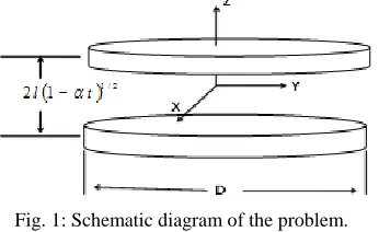
II. F

ORMULATION OF THE PROBLEM

Let the position of the two plates be at _ _1/ 2

1

z l t , where l is the position at time t = 0 as shown in below figure.

Fig. 1: Schematic diagram of the problem.

(2)

(IJSTE/ Volume 2 / Issue 08 / 015)

att 1 /



. When



is negative, the two plates are separated. Let u, v and w be the velocity component in the x, y and z directions. For two-dimensional flow, Wang introduced the following transform [8].

 

'

1/ 2

( ),

2 (1 )

( ),

2 (1 )

x

u f n

t l

w f n

t           

  ₍₁₎ Where





.

) 1 ( t 1/2 l z n    (2)

Substitute (1) into unsteady two-dimensional Navier-Stokes equations yields non-liner ordinary differential equation in form:

(3)

Where 2

/ 2

Sal v (squeeze number) is the nondimensional parameter. The flow is characterized by this parameter. The

boundary conditions are such that on the plates the lateral velocities are zero and the normal velocity is equal to the velocity of the plates, that is,

, 0 ) 0

( 

f f ''(0)0,f(1)1,f'(1)0,₍₄₎ Similarly Wang’s Transform [36] for axisymmetric flow are,

    ' ' 1/ 2 ( ),

4 (1 )

( ),

4 (1 )

( ),

2 (1 )

x

u f n

t y

v f n

t l

w f n

t                  (5)

Using transform (5), unsteady axisymmetric Navier- Stokes equation reduce to





'''' ''' '' '''

3 0,

f S nf  f ff 

(6) Subject to boundary condition (4) ,Consequently we solve nonlinear ordinary differential equation





'''' ''' '' ' '' '''

3 0

f S nf  f f f ff 

, (7) Where

0, ,

1, dim ,

Axisym m tric Tw o ensional

  



 ₍₈₎

And subject to boundary conditions (4).

III. Q

UINTIC

S

PLINE COLLOCATION METHOD

Consider equally spaced knots of partition π:ax₀ x₁ x₂ ... x_n b on__{a b}_, _. The Quintic Spline[15] is

 

_

              1 0 5 4 0 0 3 0 0 2 0 0 0 0

0 ( )

120 1 ) ( 24 1 ) ( 6 1 ) ( 2 1 ) ( n k k

k x x

F x x e x x d x x c x x b a x s (9) Where the powers function(xx_k)_ is defined as

, ( ) 0, k k k k

x x x x x x x x        _

 ₍₁₀₎ Consider a fourth -order linear boundary value problem of the form

, ), ( ) ( ) ( ) ( ) ( ) ( ) ( ) ( )

(x y x q x y x r x y x t x y x m x a x b p

yiv           ₍₁₁₎

Subject to boundary conditions

, , , , 3 '' ' 3 3 3 '' ' 0 3 2 '' ' 2 2 2 0 2 1 '' ' 1 1 1 0 1 0 '' ' 0 0 0 0 0                                            n n n n n n n n n n n n y y y y y y y y y y y y y y y y (12)

Wherey x( ),p x( ), q x( ), r x( ),t x( ) andm x( ) are continuous function defined in the interval x[ , ];a b    0, 1, 2, 3are finite real

(3)

Let (9) be an approximation solution of (11), where

0, 0, 0, 0, 0, 0, 1, ..., n1

a b c d e F F F_ are real coefficient to be determined. Let

0, 1, ..., n

x x x ben1 grid points in the interval[ , ]a b , so that

, ih a

xi   i0,1,2,...,n; x0a,xn b,

.

n a b h 

(13) It is required that approximate solution (9) satisfies the differential equation at the pointx  x_i.

Putting (9) with its successive derivatives in (11), we obtain the collocation equations as follows:

 

 



( ) ( )( ) (( )) ( ), 0,1,2,..., . ) )( ( 2 1 ) )( ( ) ( 3 ) )( ( 6 1 ) )( ( 2 1 ) )( ( ) ( ) )( ( 24 1 ) )( ( 6 1 ) )( ( 2 1 ) )( ( 1 ) )( ( 120 1 ) )( ( 24 1 ) )( ( 6 1 ) )( ( 2 1 0 0 0 2 0 0 0 0 2 0 0 0 4 0 3 0 2 0 0 0 5 4 3 2 1 0 n i x m x t a x x x t x r b x x x t x x x r x q c x x x t x x x r x x x q x p d x x x t x x x r x x x q x x x p e x x x t x x x r x x x q x x x p x x F i i i i i i i i i i i i i i i i i i i i i i i i i k i i k i i k i i k i i k i n k k                                                 



(14) From boundary conditions,

 

1

2 3 2

0 0 0

0 0

0

0 0 0 0 0 0 0 0 0 0 ,

( ) ( ) ( ) ( )

2 6 2

( ) ( ) ( ) ( )

n

k k k

k

F b x b x e b a b a

d b a c b a

               _ _ _ _  _ _ _                



1

2 3 5 2 4

1 1 1 1 1

0 1

0

3 2

1 1

0 1 1 0 1 0 1 1 0 1 1,

( ) ( ) ( ) ( ) ( ) ( )

2 6 1 2 0 2 2 4

( ) ( ) ( ( ) ) ( ( ) ) ( )

6 2

n

k k k k

k

F b x b x b x e b a b a b a d b a b a c b a b b a a

                                              _     _         



1

2 3 5 2 4

2 2 2 2 2

0 2

0

3 2

2 2

0 2 2 0 2 0 2 2 0 2 2 ,

( ) ( ) ( ) ( ) ( ) ( )

2 6 1 2 0 2 2 4

( ) ( ) ( ( ) ) ( ( ) ) ( )

6 2

n

k k k k

k

F b x b x b x e b a b a b a

d b a b a c b a b b a a

                     _ _ _ _ _ _  _ _ _ _ _             _     _         



1

2 3 5 2 4

3 3 3 3 3

0 3

0

3 2

3 3

0 3 3 0 3 0 3 3 0 3 3 ,

( ) ( ) ( ) ( ) ( ) ( )

2 6 1 2 0 2 2 4

( ) ( ) ( ( ) ) ( ( ) ) ( )

6 2

n

k k k k

k

F b x b x b x e b a b a b a d b a b a c b a b b a a

                                              _     _           (15)

Using the power function(xx_k)_ in the above equations, a system ofn5 linear equations inn5 unknowns 0, 0, 0, 0, 0, 0, 1, ..., n 1

a b c d e F F F is thus obtained. This system can be written in matrix vector form as follows:A X  B.

Where [ 1, 2 ,, ..., 2, 1, 0, 0, 0, 0, 0, 0] , [ 3, 2, 1, 0, ( ), ( 1), ..., ( 0)] .

T T

n n n n

X  F_ F_ F F F e d c b a B     m x m x_ m x

The coefficient matrix A is an upper triangular Hessen berg matrix with single lower sub diagonal, principal and upper diagonal having non zero element, because of this nature of a matrix A, the determination of the required quantities becomes simple and consumes less time. The values of these constants ultimately yield the quintic spline s(x) in (9).

In case of nonlinear boundary value problem, the equations can be converted into linear form using Quasilinearization method (Bellman and Kalaba [14]), and hence this method can be used as iterative method. The procedure to obtain a spline

approximation ofy_i (i=0, 1, 2,…., j, where j denotes the number of iteration) by an iterative method starts with fitting a curve satisfying the end conditions and this curve design asy_i. We obtain the successive iterationy_i’s with the help of the algorithm described as above till desired accuracy.

IV. S

OLUTION BY USING COLLOCATION METHOD

In order to solve equation (3) using conditions (4), we use quasilinearization technique to convert into linear form.

'''' ''' '' '' ' ''' '' ' '''

1 1 1 1

( ) ( 3 ) ( )

i i i i i i i i i i i i i

f  ssf f_   ssf f_  sf f_ sf f_  sf f sf f

(16) Consider the quintic spline is an approximate solution of equation (16)

 

2 3 4 1 5

0 0 0 0 0 0 0 0 0

0

1 1 1 1

( ) ( ) ( ) ( ) ( )

2 6 24 120

n

k k k

s  a b   c   d   e   F  



 

(4)

For finding the initial value of fi, ,we assume f n_i( )a3b2cdto be the first approximation to start the iterative

scheme, which satisfy the given conditions. As discussed in above method, substitute equation (17) with its derivatives in equation (16), we obtain collocation equation as:

' '' '''

1

2 3 4 5

0

' '' '''

2 3 4

0 0 0 0 0

0

( ) ( 3 ) ( ) ( )

[( ) ( ) ( ) ( ) ( ) ]

2 6 2 4 1 2 0

( 3 ) ( ) ( )

[1 ( )( ) ( ) ( ) ( ) ]

2 6 2 4

[( ) ( 3

n

i i i i

k i k i k i k i k i k

k

i i i

i i i i i

i

s sf s sf sf sf F

s sf sf sf e s sf

d s sf s

  

         

 

        

 





    

        

  

          

     



'' '''

' 2 3

0 0 0

'''

' '' 2

0 0 0

'' '''

0 0

''' '' ' '''

0

( ) ( )

)( ) ( ) ( ) ]

2 6

( )

[( 3 ) ( )( ) ( ) ]

6

[( ) ( )( )]

[( )]

i i

i i i i

i

i i i i

i i i

i i i i i

sf sf sf

sf c s sf sf

b sf sf

a sf sf f sf f



     

     

  





    

       

   

    ₍₁₈₎

Substitute initial conditions in ( )s  , and we get following equations

0

0 0 0 0 0 0 1 2 3 4

0 0 0 0 0 1 2 3

0,

(0.5) (0.1666) (0.041666) (0.008333) (0.0002 73) (0.000647 ) (0.00000853) (0.00000266) 1,

(0.5) (0.16667 ) (0.041666) (0.0170666) (0.00 054) (0.0001066) 0. a

c

a b c d e f f f f f

b c d e f f f f

 

         

       

(19)

Solve above equations and substitute constants in (17) and we get the solution for different values of S and 1

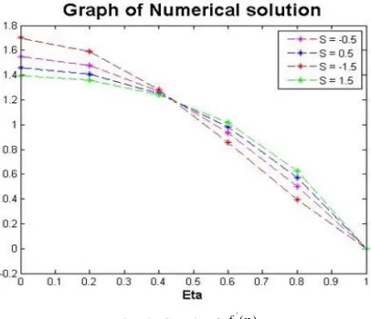
Graphical Solution of Given Problem

Fig. 2: Graph of Analytical Solution Fig. 3: Graph of Numerical Solution

Graph of f'( )

Fig. 4: Graph of

'

( )

(5)

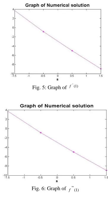
Graph of f'''(1)

Fig. 5: Graph of f'''(1)

Graph of f'''(1)

Fig. 6: Graph of _f'''₍₁₎

V. R

ESULT AND DISCUSSION

In this section, comparisons of results are made through different squeeze numbers S, All Computations are performed numerically by quintic spline collocation method. The numerical results are agreed with the available analytical solutions. From

the figure (ii), the velocity increases due to an increase in S. Figures (ii) & (iii) shows comparison of f( ) and f



'

 



with increase in S. These quantities describe the flow behavior, f'''(1) gives skin frication and f '''(1)represents pressure gradient,

'''

(1)

f and '''

(1)

f as a function of S are shown in figures (iv) & (v).

VI. C

ONCLUSION

There are two important goals that we have fulfilled for this study. The first one is to employ successfully the spline collocation method to investigate the behavior of two dimensional squeezing flows between two parallel plates and second is to investigate the influence of the squeeze number on the velocity, skin friction and pressure gradient. Here, the results are compared with HPM. The obtained solutions, in comparison with the numerical solutions, demonstrate remarkable accuracy.

R

EFERENCES

[1] M. J. Stefan, “ Versuch Uber die scheinbare adhesion , “ Sitzungsberichten der Akademie der Wissenschaften in Wien, Mathematische

Naturwissenschaften, vol. 69,pp. 713-721, 1874.

[2] O. Reynolds, “On the theory of lubrication, “Transactions of the Royal Society, vol. 177, no.1, pp.157-234, 1886.

[3] F. R. Archibald, “Load capacity and time relations in squeeze films, “Transactions of the ASME, Journal of Lubrication Technology, vol. 78, pp. 29-35,

1956.

[4] C. Y. Lai, K. R. Rajagopal, and A. Z. Szeri, "Asymmetric ﬂow between parallel rotating disks," The Journal of Fluid Mechanics, vol. 146, p. 203, 1984.

[5] C. Y. Lai, K. R. Rajagopal, and A. Z. Szeri, "Asymmetric ﬂow above a rotating disk," Journal of Fluid Mechanics, vol. 157, pp. 471-492, 1985.

[6] Al- Said, E.A. and Noor, M.A. “Numerical solution of a system of fourth order boundary value problems”, International Journal of Computer Mathematics,

70, pp. 347-355 (1998).

[7] Aziz, T. and Khan, A. “Quintic spline approach to the solution of singularly perturbed boundary value problems”, Journal of Optimization Theory and

(6)

[8] Saeed Dinarvand and Abed Moradi, “Two-Dimensional and axisymmetric Unsteady flows due to normally Expanding or contracting Parallel Plates”,

Journal of Applied Mathematics,Volume 2012, Article ID 938624,13 pages,doi:10.1155/2012/938624.

[9] Jain, M.K., Iyengar, S.R.K. and Jain, R.K. “Numerical Methods for Scientificand Engineering Computation”, New Age International Publishers, New Delhi

(2007).

[10] Khalifa, A.K. and Noor, M.A. “Quintic spline solutions of a class of contactproblems”, Mathematical and Computer Modeling, 13, pp. 51-58 (1990).

[11] Loscalzo, F.R. and Talbot, T.D. “Spline function approximations for solutionsof ordinary differential equations”, SIAM Journal of Numerical Analysis,

4,pp. 433-445 (1967).

[12] Noor, M.A. and Al- Said, E.A. “Numerical solution of fourth order variationalinequalities”, International Journal of Computer Mathematics, 75, pp.

107-116(2000).

[13] G. Micula and S. Micula, Handbook of splines, kluwer Academic Publisher, Dordrecht, The Netherlands, 1998.

[14] R. E.Bellman and R. E. Kalaba, Quasilinearization and Nonlinear Boundary-Value Problems, American Elsevier Publishing Co, New York, NY, USA,

1965.