ISSN (e): 2250-3021, ISSN (p): 2278-8719
Vol. 05, Issue 08 (August. 2015), ||V3|| PP 45-51
Numerical Solution of a Linear Black-Scholes Models: A
Comparative Overview
Md. Kazi Salah Uddin, Md. Noor-A-Alam Siddiki, Md. Anowar Hossain
Department of Natural Science, Stamford University Bangladesh, Dhaka-1209, Bangladesh.Abstract: - Black-Scholes equation is a well known partial differential equation in financial mathematics. In this paper we try to solve the European options (Call and Put) using different numerical methods as well as analytical methods. We approximate the model using a Finite Element Method (FEM) followed by weighted average method using different weights for numerical approximations. We present the numerical result of semi-discrete and full semi-discrete schemes for European Call option and Put option by Finite Difference Method and Finite Element Method. We also present the difference of these two methods. Finally, we investigate some linear algebra solvers to verify the superiority of the solvers.
Keywords: Black-Scholes model; call and put options; exact solution; finite difference schemes, Finite Element Methods.
I.
INTRODUCTION
A powerful tool for valuation of equity options is the Black-Scholes model[12,15]. This model is used for finding the prices of stocks.
R. Company, A.L. Gonzalez, L. Jodar [14] solved the modified Black-Scholes equation pricing option with discrete dividend.
A delta-defining sequence of generalized Dirac-Delta function and the Mellin transformation are used toobtain an integral formula. Finally numerical quadrature approximation is used to approximate the solution.
In some papers like [13] Mellin transformation is used. They were required neither variable transformation nor solving diffusion equation.
R. Company, L. Jodar, G. Rubio, R.J. Villanueva [13] found the solution of BS equation with a wide class of payoff functions that contains not only the Dirac delta type functions but also the ordinary payoff functions with discontinuities of their derivatives.
Julia Ankudiova, Matthias Ehrhardt [20] solved non linear Black-Scholes equations numerically. They focused on various models relevant with the Black-Scholes equations with volatility depending on several factors. They also worked on the European Call option and American Call option analytically using transformation into a convection -diffusion equation with non-linear term and the free boundary problem respectively.
In our previous paper [7] we discussed about the analytical solution of Black-Scholes equation using Fourier Transformation method for European options. We formulated the Finite Difference Scheme and found the solutions of them.
In this paper we discuss the solution with Finite Element Method and compare the result with the result obtained by Finite Difference Schemes.
II.
MODEL EQUATION
The linear Black-Scholes equation [12,15] developed by Fischer Black and Myron Scholes in 1973 is 𝑉𝑡+ 𝑟𝑆𝑉𝑆+
1 2𝜎
2𝑆2𝑉
𝑆𝑆− 𝑟𝑉 = 0 … … … (1)
where
𝑉 = 𝑉 𝑆, 𝑡 , 𝑡ℎ𝑒 𝑝𝑎𝑦 − 𝑜𝑓𝑓 𝑓𝑢𝑛𝑐𝑡𝑖𝑜𝑛 𝑆 = 𝑆(𝑡), 𝑡ℎ𝑒 𝑠𝑡𝑜𝑐𝑘 𝑝𝑟𝑖𝑐𝑒, 𝑤𝑖𝑡ℎ 𝑆 = 𝑆(𝑡) ≥ 0, 𝑡 = 𝑡𝑖𝑚𝑒, 𝑟 = 𝑅𝑖𝑠𝑘 − 𝐹𝑟𝑒𝑒 𝑖𝑛𝑡𝑒𝑟𝑒𝑠𝑡 𝑟𝑎𝑡𝑒, 𝜎 = 𝑉𝑜𝑙𝑎𝑡𝑖𝑙𝑖𝑡𝑦 𝐶𝑜𝑛𝑑𝑖𝑡𝑖𝑜𝑛
and also 𝑡 ∈ (0, 𝑇). where T is time of maturity.
European Call Option [16]
The solution to the Black-Scholes equation (1) is the value 𝑉(𝑆, 𝑡) of the European Call option on $0 ≤ 𝑆 <
∞, 0 ≤ 𝑡 ≤ 𝑇. The boundary and terminal conditions are as follows
𝑉 0, 𝑡 = 0 𝑓𝑜𝑟 0 ≤ 𝑡 ≤ 𝑇,
𝑉 𝑆, 𝑡 ∼ 𝑆 − 𝐾𝑒−𝑟 𝑇−𝑡 𝑎𝑠 𝑆 →∞,… … … (2)
𝑉 𝑆, 𝑇 = 𝑆 − 𝐾 + 𝑓𝑜𝑟 0 ≤ 𝑆 <∞.
European Put Option[16]
European Put option is the reciprocal of the European Call option and the boundary and terminal conditions are
𝑉 0, 𝑡 = 𝐾𝑒−𝑟 𝑇−𝑡 𝑓𝑜𝑟 0 ≤ 𝑡 ≤ 𝑇,
𝑉 𝑆, 𝑡 → 0 𝑎𝑠 𝑆 →∞,… … … (3) 𝑉 𝑆, 𝑇 = 𝐾 − 𝑆 + 𝑓𝑜𝑟 0 ≤ 𝑆 <∞.
III.
TRANSFORMATION
The model problem stated in (1) is a backward type. This type is little bit difficult to solve. To solve the problem in (1) with the conditions stated in (2) and (3) we need to make the model in forward type. In this regard, we have the following transformations.
Let
𝑆 = 𝐾𝑒𝑥
𝑡 = 𝑇 − 𝜏
𝜎2 /2 And
𝑣(𝑥, 𝜏) =1 𝐾𝑉(𝑆, 𝑡) 𝜕𝑉 𝜕 𝑡 = 𝜕𝑉 𝜕𝜏 𝜕𝜏 𝜕𝑡+ 𝜕𝑉 𝜕𝑆𝜕𝑆 𝜕𝑡 = −𝜎 2
2 𝐾 𝜕𝑣 𝜕𝜏 𝜕𝑉 𝜕𝑆 = 𝐾 𝜕𝑣 𝜕𝑆= 𝐾 𝑆 𝜕𝑣 𝜕𝑥 𝜕2𝑉
𝜕𝑆2 = 𝐾
𝜕2𝑣
𝜕𝑆2=
𝐾 𝑆2
𝜕2𝑣
𝜕𝑥2−
𝜕𝑣 𝜕𝑥
inserting these derivatives in equation (1) we have
−𝜎
2
2 𝐾 𝜕𝑣 𝜕𝜏+
𝜎2
2 𝐾 𝜕2𝑣
𝜕𝑥2−
𝜕𝑣 𝜕𝑥+ 𝑟𝐾
𝜕𝑣
𝜕𝑥− 𝑟𝐾𝑣 = 0.
implies
𝜕𝑣 𝜕𝜏 =
𝜕2𝑣
𝜕𝑥2+
𝑟 𝜎2
2
− 1 𝜕𝑣 𝜕𝑥−
𝑟 𝜎2
2
𝑣 … … … (4)
Let
𝑟 𝜎2
2 = 𝜃
∴ (4) implies
𝜕𝑣 𝜕𝜏=
𝜕2𝑣
𝜕𝑥2+ 𝜃 − 1
𝜕𝑣
𝜕𝑥− 𝜃𝑣. … … … . . (5)
Now let
𝜆 =1
2(𝜃 − 1), 𝜈 = 1
2(𝜃 + 1) = 𝜆 + 1 so that
𝜈2= 𝜆2+ 𝜃
𝑣(𝑥, 𝜏) = 𝑒−𝜆𝑥 −𝜈2𝜏
𝑢(𝑥, 𝜏). 𝜕𝑣
𝜕𝜏 = 𝑒
−𝜆𝑥 −𝜈2𝜏 −𝜈2 𝑢 𝑥, 𝜏 +𝜕𝑢
𝜕𝜏𝑒
−𝜆𝑥 −𝜈2𝜏
= 𝑒−𝜆𝑥 −𝜈2𝜏[−𝜈2𝑢 +𝜕𝑢 𝜕𝜏],
𝜕𝑣
𝜕2𝑣
𝜕𝑥2= 𝑒 −𝜆𝑥 −𝜈2𝜏
[𝜆2𝑢 − 2𝜆𝜕𝑢
𝜕𝑥+ 𝜕2𝑢
𝜕𝑥2]. inserting these into equation(5) and dividing by 𝑒−𝜆𝑥 −𝜈2𝜏we get
−𝜈2𝑢 +𝜕𝑢
𝜕𝜏 = [𝜆
2𝑢 − 2𝜆𝜕𝑢
𝜕𝑥+ (𝜕
2𝑢)/(𝜕𝑥2)] + (𝜃 − 1)[−𝜆𝑢 +𝜕𝑢
𝜕𝑥] − 𝜃𝑢
implies
𝑢𝜏= 𝑢𝑥𝑥 + −2𝜆 + 𝜃 − 1 𝑢𝑥+ (𝜆2+ 𝜈2− 𝜆(𝜃 − 1))𝑢
= 𝑢𝑥𝑥.
∴ 𝑢𝜏= 𝑢𝑥𝑥… … … (6)
And the initial & boundary conditions for the European Call and Put options are respectively
𝑢 𝑥, 0 = 𝑒 𝜆+1 𝑥− 𝑒𝜆𝑥 + 𝑎𝑠 𝑥 ∈ ℝ
𝑢 𝑥, 𝜏 = 0 𝑎𝑠 𝑥 → −∞
𝑢 𝑥, 𝜏 = 𝑒 𝜆+1 𝑥+𝜈2𝜏
− 𝑒𝜆𝑥 +𝜆2𝜏
𝑎𝑠 𝑥 →∞
… … … . . … … … . (7)
and
𝑢 𝑥, 0 = 𝑒𝜆𝑥− 𝑒 𝜆+1 𝑥 + 𝑎𝑠 𝑥 ∈ ℝ
𝑢 𝑥, 𝜏 = 𝑒𝜆𝑥 +𝜆2𝜏 𝑎𝑠 𝑥 → −∞… … … . . … … … . (8)
𝑢 𝑥, 𝜏 = 0 𝑎𝑠 𝑥 →∞
Thus the Black-Scholes equation reduced to a heat diffusion equation.
IV.
NUMERICAL APPROXIMATION OF TRANSFORMED LINEAR
BLACK-SCHOLES MODEL
Now we solve the problems numerically. We use the Finite Element Method (FEM) to solve the problems related to the differential equation (6). Finally back substitution of the coordinate transformation gives the solution of the problems related to the differential equation (1).
We have the model
𝑢𝜏= 𝑢𝑥𝑥, 𝑥 ∈ ℝ, 0 ≤ 𝜏 ≤ 𝑇 .… … … (9) and the initial and boundary conditions for call option are
𝑢 𝑥, 0 = 𝑒 𝜆+1 𝑥− 𝑒𝜆𝑥 + 𝑎𝑠 𝑥 ∈ ℝ,
𝑢 𝑥, 𝜏 = 0 𝑎𝑠 𝑥 → −∞… … … . . (10) 𝑢 𝑥, 𝜏 = 𝑒 𝜆+1 𝑥+𝜈2𝜏− 𝑒𝜆𝑥 +𝜆2𝜏 𝑎𝑠 𝑥 →∞
The weak form of the governing equation is 𝜕𝑢 𝜕𝜏 ℝ 𝑣(𝑥)𝑑𝑥 + 𝜕𝑢 𝜕𝑥 𝜕𝑣 𝜕𝑥𝑑𝑥
ℝ = 0… … … . (11) Since 𝑣 𝑥 → 0 as 𝑥 → ±∞.
Discretizing 𝑢(𝑥, 𝜏) spatially, we have
𝑢 𝑥, 𝜏 = 𝜙𝑖 𝜏 𝑁𝑖 𝑥 𝑛
−𝑛
… … … . (12)
where 𝑁𝑖(𝑥) are given shape functions, and 𝜙𝑖(𝜏) are unknown, and 𝑛 is the ordinal number of nodes. Substituting (12) into (11), we get the weak semidiscretized equation
𝜙𝑖′ 𝜏 𝑁𝑖 𝑥 𝑁𝑗(𝑥)𝑑𝑥 1 0 𝑛 −𝑛 + 𝜙𝑖 𝜏 𝑁′𝑖 𝑥 𝑁′𝑗(𝑥)𝑑𝑥 1 0 𝑛 −𝑛
= 0 … … … . . (13)
Let 𝑄, 𝑀 ∈ ℝ 2𝑛−1 × 2𝑛−1 denote the so-called mass and stiffness matrices, respectively, defined by:
𝑀𝑖𝑗 = 𝑁′𝑖 𝑥 𝑁′𝑗(𝑥)𝑑𝑥 1
0
… … … . . (14)
𝑄𝑖𝑗 = 𝑁𝑖 𝑥 𝑁𝑗(𝑥)𝑑𝑥 1
0
… … … . . … … . . (15)
Then (13) can be expressed as:
𝑄𝛷′+ 𝑀𝛷 = 0 … … … . (16)
where Φ∈ ℝ2𝑛−1 is a vector function with the components 𝜙 𝑖.
𝑀 =1
ℎ
−1 2 −1 … 0
⋮ ⋱ ⋱ ⋱ ⋮
0 0
…
… −10 2−1−11
; 𝑄 =6
ℎ
1 4 1 … 0
⋮ ⋱ ⋱ ⋱ ⋮
0 0
…
… 10 41 12
where ℎ is the length of the spatial approximation.
Now we would like to discrete the equation (16) with respect to time. One may start with a simple scheme. One of the trivial choice is to use the forward Euler scheme. Firstly we discrete (16) explicitly and we have
𝑄Φ′+ 𝑀Φ= 0, Φ′+ 𝑄−1𝑀Φ= 0, Φ𝑚 +1−Φ𝑚
Δ𝜏 + 𝑄
−1𝑀Φ𝑚= 0,
Φ𝑚 +1−Φ𝑚+Δ𝜏𝑄−1𝑀Φ𝑚 = 0, Φ𝑚 +1− 𝐼 −Δ𝜏𝑄−1𝑀 Φ𝑚 = 0,
Φ𝑚 +1 = 𝐼 −Δ𝜏𝑄−1𝑀 Φ𝑚. … … … . (17)
The difficulty of using the scheme is that it needs very little step size to converge , as a result the scheme is a slow one, and is not of interest in this advance study.
We want a fast and efficient scheme, so we want larger time stepping, and interested in using implicit techniques. We discrete (16) implicitly and have
Φ𝑚 +1−Φ𝑚 Δ𝜏 + 𝑄
−1𝑀Φ𝑚 +1= 0,
Φ𝑚 +1−Φ𝑚+Δ𝜏𝑄−1𝑀Φ_(𝑚 + 1) = 0,
𝐼 +Δ𝜏𝑄−1𝑀 Φ𝑚 +1=Φ𝑚,
Φ𝑚 +1= 𝐼 +Δ𝜏𝑄−1𝑀 −1Φ𝑚. … … … (18) which is a system of linear equations with unknowns Φ𝑚 +1. The advantage of using (18)
is that the scheme is unconditionally stable . Equation (18) accuracy of order 𝑂(𝑘). It is faster than the explicit Euler scheme since (18) allows us to use large time steps.
We use an weighted average method to discrete (16) with weight 𝛿 and we have Φ𝑚 +1−Φ𝑚
Δ𝜏 + 𝑄
−1𝑀(𝛿Φ𝑚 +1+ 1 − 𝛿 Φ𝑚) = 0,
Φ𝑚 +1−Φ𝑚+Δ𝜏𝑄−1𝑀(𝛿Φ𝑚 +1+ 1 − 𝛿 Φ𝑚) = 0,
𝐼 +Δ𝜏𝑄−1𝑀𝛿 Φ𝑚 +1= 𝐼 −Δ𝜏𝑄−1𝑀 1 − 𝛿 Φ𝑚,
Φ𝑚 +1 = 𝐼 +Δ𝜏𝑄−1𝑀𝛿 −1 𝐼 −Δ𝜏𝑄−1𝑀 1 − 𝛿 Φ𝑚. … … … . . (19) This system is also a linear one with unknowns Φ𝑚 +1, where 𝛿 varies from 0 to 1. This
method turns to the explicit method when 𝛿 = 0 i.e., equations (17) and (19) are same and implicit method when 𝛿 = 1, i.e., equations (18) and (19)are same. For 0 ≤ 𝛿 ≤1
2, the scheme is conditionally stable and unconditionally stable for 1
2≤ 𝛿 ≤ 1.
The order of the accuracy of the scheme is 𝑂(𝑘).
V.
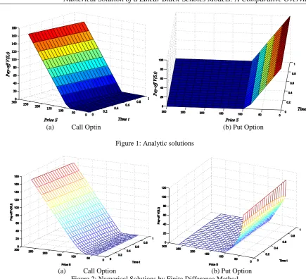
RESULTS, DISCUSSION AND CONCLSTION
(a) Call Optin (b) Put Option
Figure 1: Analytic solutions
(a) Call Option (b) Put Option
Figure 2: Numerical Solutions by Finite Difference Method
(a) Call Option (b) Put Option
Figure 4: Comparison of Finite Difference Method and Finite Element Method
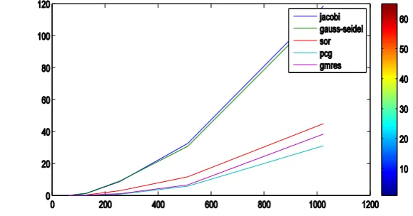
The system of linear equations (19) generated by the discretization of the Black-Scholes model can be solved by many conventional processes. For a large scale linear system, scientists rarely use direct methods as they are computationally costly. Here, in this section, it is our motivation to solve the system of equation (19) using various iterative techniques. Here we first investigate which linear solver converges swiftly. To that end, we consider Jacobi iterative method, Gauss-Seidel iterative method and successive over relaxation method to start with. In terms of matrices, the Jacobi method can be expressed as
x(k) = D−1 L + U x(k−1) + D−1b, Gauss-Seidel method
x(k) = D − L −1(Ux k−1 + b),
and the SOR algorithm can be written as
x k = D −ωL −1 ωU + 1 −ω D x k−1 +ω D −ωL −1b,
where in each case the matrices D, −L, and −U represent the diagonal, strictly lower triangular, and strictly upper triangular parts of A, respectively.
Figure 5: Time comparison of different linear algebra solvers
REFERENCES
[1] P. E. Lewis and J. P. Ward, The Finite Element Method: Principles and Applications, ADDISONWESLEY PUBLISHING COMPANY, 1991.
[2] M. Bakker, One-dimensional Galerkin methods and super convergence at interior nodal points, SIAM Journal on Numerical Analysis, 21(1):101–110, Feb 1984.
[3] S. K. Bhowmik, Stable numerical schemes for a partly convolutional partial integrodifferential equation, Applied Mathematics and Computation, 217(8):4217–4226,2010.
[4] S. K. Bhowmik,Numerical approximation of a convolution model of dot theta-neuron networks, Applied Numerical Mathematics, 61:581–592, 2011.
[5] S. K. Bhowmik, Stability and convergence analysis of a one step approximation of a linear partial integro- differential equation, Numerical Methods for Partial Differential Equation, 27(5):11791200, September 2011.
[6] S. K. Bhowmik, Fast and efficient numerical methods for an extended Black-Scholes model,arXiv:1205.6265, 2013.
[7] Md. Kazi Salah Uddin, Mostak Ahmed and Samir Kumar Bhowmik, A Note On Numerical Solution Of A Linear Black-Scholes Model, GANIT J. Bangladesh Math. Soc. (ISSN 1606-3694), Vol. 33 (2013) 103- 115.
[8] Cristina Ballester, Rafael Company*, Lucas Jodar, An efficient method for option pricing with discrete dividend payment, Computers and Mathematics with Applications, 2008, Vol.56, pp. 822-835.
[9] A.H.M. Abdelrazec, Adomain Decomposition Method: Convergency Analysis and Numerical Approxima- tion, McMaster University, 2008.
[10] Koh Wei Sin, Jumat Sulaiman and Rasid Mail, Numerical Solution for 2D European Option Pricing Using Quarter-Sweep Modified Gauss-Seidel Method, Journal of Mathematics and Statistics8 (2012), no. 1, 129-135.
[11] H.W. Choi and S.K. Chung, Adaptive Numerical Solutions For The Black-Scholes Equation, J. Appl. Math. & Computing (Series A), Vol. 12, No. 1–2, pp.335–349, 2003.
[12] R.C. Merton, Theoryof rational option pricing, Bell J. Econ., Vol. 4, No. 1, pp.141–183, 1973.
[13] L. Jodar, R Sevilla-Peris, J.C. Cortos*, R. Sala, A new direct method for solving the Black-Scholes equation, Applied Mathematics Letters, Vol. 18, pp.29–32, 2005.
[14] R. Company*, A.L. Gonzalez, L. Jodar, Numerical solution of modified Black–Scholes equation pricing stock options with discrete dividend, Mathematical and Computer Modelling, Vol. 44, pp.1058–1068, 2006.
[15] F. Black, M. Scholes, The pricing of options and corporate liabilities, J. Pol. Econ, Vol. 81, pp.637–659, 1973.
[16] P.D.M. Ehrhardt and A. Unterreiter, The numerical solution of nonlinear Black–Scholes equations, Technische Universitat Berlin, Vol. 28, 2008.
[17] M. Bohner and Y. Zheng, On analytical solutions of the Black-Scholes equation, Applied Mathematics Letters, Vol. 22, pp.309–313, 2009.
[18] John C.Strikwerda, Finite Difference Schemes and Partial Differential Equations, SIAM,University of Wisconsin-Madison Madison, Wisconsin, 2004.
[19] Julia Ankudinova*, Matthias Ehrhardt, On the numerical solution of nonlinear Black–Scholes equations, Computers and Mathematics with Applications, Vol. 56, pp.799-812, 2004.
[20] D.J. Duffy, Finite Difference Methods in Financial Engineering (A Partial Differential Equation Ap-proach), John Wiley & Sons Ltd, The Atrium, Southern Gate, Chichester, West Sussex PO19 8SQ, England, 2000.