Studies on Optimization Algorithms for Some
Artificial Neural Networks Based on Genetic
Algorithm (GA)
Shifei Ding1, 2, Xinzheng Xu1, Hong Zhu1 1
School of Computer Science and Technology, China University of Mining and Technology, Xuzhou 221116; 2
Key Laboratory of Intelligent Information Processing, Institute of Computing Technology, Chinese Academy of Science, Beijing, 100080
Email: [email protected], [email protected]
Jian Wang, Fengxiang Jin
Geomatics College, Shandong University of Science and Technology, Qingdao 266510
Abstract—Artificial Neural Networks (ANNs) are the
nonlinear and adaptive information processing systems which are combined by numerous processing units, with the characteristics of self-adapting, self-organizing and real-time learning, and play an important in pattern recognition, machine learning and data mining. But we’ve encountered many problems, such as the selection of the structure and the parameters of the networks, the selection of the learning samples, the selection of the initial values, the convergence of the learning algorithms and so on. Genetic algorithms (GA) is a kind of random search algorithm, on one hand, it simulates the nature selection and evolution, on the other, it has the advantages of good global search abilities and learning the approximate optimal solution without the gradient information of the error functions. In this paper, some optimization algorithms for ANNs with GA are studied. Firstly, an optimizing BP neural network is set up. It is using GA to optimize the connection weights of the neural network, and using GA to optimize both the connection weights and the architecture. Secondly, an optimizing RBF neural network is proposed. It used hybrid encoding method, that is, to encode the network by binary encoding and the weights by real encoding, the network architecture is self-adapted adjusted, the weights are learned, and the network is further adjusted by pseudo-inverse method or LMS method. Then they are used in real
world classification tasks, and compared with the
modified BP algorithm with adaptive learning rate. Experiments prove that the network got by this method has a better architecture and stronger classification ability, and the time of constructing the network artificially is saved. The algorithm is a self-adapted and intelligent learning algorithm.
Keywords- Artificial neural networks (ANNs); BP network; RBF network; Genetic Algorithm (GA); Network Structure; Network Weight
I. INTRODUCTION
Artificial Neural Networks (ANNs)[1] are the nonlinear and adaptive information processing systems which are combined by numerous processing units, with the characteristics of self-adapting, self-organizing and real-time learning. From 1980s, the research of ANNs has obtained notable developments, and ANNs have been widely applied to pattern recognition, machine learning, data mining, and so on. However, with the development of the research, we’ve encountered many problems, such as the selection of the structure and the parameters of the networks, the selection of the learning samples, the selection of the initial values, the convergence of the learning algorithms and so on.
It is known that the performance of ANNs is sensitive to the number of neurons. Too few neurons can result in poor approximation, while too many neurons may contribute to overfitting problems. Obviously, achieving a better network performance and simplifying the network topology are two competing objectives. From 1990s, Evolution Algorithms (EAs) have been successfully used in optimizing the design and the parameters of ANNs [2].
Back-propagation (BP) neural network is one of the most maturely studied neural network algorithms. A three-layered BP neural network can approach any non-linear function with any precision [3]. BP neural network has been widely applied in many fields, such as pattern recognition, function approximation and image processing etc.
However, BP algorithm has its disadvantages: slow convergence speed; east to get stuck in local minimum; a good network architecture need to be tried. Many optimization algorithms have been introduced to the learning and design of neural networks to overcome those above problems, such as: constructing a neural network based on particle swarm optimization algorithm [4]; using
evolutionary algorithms to optimize the neural network architecture [5-7]. They have been proved to be feasible and effective.
The differences between Radial Basis Function (RBF) neural network and three-layer perception are: RBF neural network has only one group of weights (from hidden to output layer); RBF neural network use both supervised and unsupervised learning; the transfer functions are different (RBF neural network uses Gaussian radial basis function). In the hidden layer of RBF neural network, each node is corresponding to a center (a vector that has the same length of the sample), the centers are usually got by K-Mean cluster (unsupervised learning), the weights of output layer are got by pseudo inverse method. RBF neural network has been widely applied in the traditional classification problems [8]. Research showed that the nonlinear transfer functionsused by RBF neural networks do not influence the network performance very much, the key is the selection of basis function centers. Two many centers will lead to over-fitting while too few centers will lead to poor classification ability [9]. For the shortages of common RBF learning algorithms (randomly choosing some data as centers and learning the weights by pseudo inverse method), S. Chen et al.[10] proposed an improved algorithm based on orthogonal least squares (OLS) method, which chooses RBF centers in a rational way until an adequate network has been constructed. D. Venkatesan et al.[11] pointed out that the learning of neural network is time-consuming; thereby using Genetic Algorithm to construct the model can get more accurate results with less time consumed. GA is used to optimize BP neural network much more than RBF, so C. Venkatesan et al.[12] made a survey on using GA in the learning of RBF neural network. X. Yao[13] made a survey on using evolutionary algorithms to optimize neural network learning, he named this evolutionary neural network. In this paper an optimizing algorithm of RBF neural network based on GA is proposed; it used hybrid encoding method, that is, to encode the network by binary encoding and the weights by real encoding; the network architecture is self-adapted adjusted and the weights are learned.
From 1990s, Evolution Algorithms(EAs) have been successfully used in optimizing the design and the parameters of ANNs. EAs is a kind of random search algorithm which simulates the nature selection and evolution [14]. It has the advantages of good global search abilities and learning the approximate optimal solution without the gradient information of the error functions. By its special nature evolution rules and superiority of population optimizing search, EAs provides new ideas and methods for solving problems.
EAs mainly include Evolutionary Strategy (ES), Evolutionary Programming (EP) and Genetic Algorithm (GA). The three evolutionary algorithms are accordant on the goal of using biological evolution mechanism to improve the ability of using computers to solve problems, but they are different on the concrete measure: ES stress the behavior change of individual level, EP stress the
behavior change of population level, and GA stress the operation to the chromosome. In addition to this, there’re also Genetic Programming, Memetic Algorithm, etc [15].
GA is an important branch of EAs. It draws lessons from the theory of biological evolution which is “selecting the superior and eliminating the inefficient, survival of the fittest”. After select, crossover and mutate from one generation to another, the population tends to a balance state where some features have relative potency. GA starts from a population that represents the hidden solution set of the problem; the solution set is composed by a designated number individual got by gene coding. In fact each individual is the substance of some chromosome with features. A chromosome is the set of several genes, so at first it is need to implement the mapping from phenotype to genotype by coding. In each generation of evolvement, GA selects the individuals according to their fitness, then crossovers and mutates to generate a new population of the solution set. At last GA can get the approximate optimum solution from the decoding result of the optimum individual of the final population. In practical problems, the coding methods of the feasible solution and the design of genetic operators are the two main problems when constructing GA; different problems may use different coding methods and different genetic operators.
Currently, computation intelligence is in the stage of rapid growth, its main techniques include fuzzy technology, neural network, evolutionary algorithm, etc. With the development of computer techniques, these methods have achieved big progress and tended to integrate together. They can reinforce them by the mutual complementation, so as to gain more powerful abilities of representing and solving the practical problems. EAs and ANNs both are the theoretical results of applying biological principles to the science research. More and more researchers try to combine EAs and ANNs in recent years [16], hope to combine their advantages, so as to find a more efficient method. This is mainly manifested in using EAs to optimize the network design, pre-processing the network input data, the assemble of ANNs[17], etc. This paper organizes as follows. In Section Ⅱ, two typical ANNs, includes BP network and RBF network are introduced, meanwhile the principle of EAs, specially GA, is introduced. In Section Ⅲ, some optimization algorithms are set up. Experiments are done in Section Ⅳ.
II. THEBASICPRINCIPLES
A. The Principle of BP
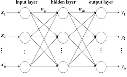
Figure 1. The architecture of BP neural network
Fig. 1 shows such a network. In the network, there is an input layer, an output layer, with one or more hidden layers in between them.
Suppose there are
n
inputs andm
outputs in the network,s
neurons in the hidden layer, the output of the hidden layer isb
j, the threshold value of the hiddenlayer is
θ
j, the threshold value of the output layer isθ
k,the transfer function of the hidden layer is
f
1, the transfer function of the output layer isf
2, the weight from input layer to hidden layer isw
ij,the weight formhidden layer to output layer is
w
jk, then we can get theoutput of the network
y
k, the desired output ist
k, theoutput of
j
th neuron of the hidden layer is:⎟ ⎟ ⎠ ⎞ ⎜
⎜ ⎝ ⎛
−
=
∑
=
n
i
j i ij
j f w x
b
1
1
θ
(1)(
i
=
1
,
2
,
"
,
n
;j
=
1
,
2
,
"
,
s
)Calculate the output
y
kof the output layer, that is:⎟⎟ ⎠ ⎞ ⎜⎜
⎝ ⎛
−
=
∑
=
k s
j j jk k f w b
y θ
1
2 (2)
(j=1,2,",s;k=1,2,",m)
Define the error function by the network actual output, that is:
(
)
∑
=
−
=
mk
k
k
y
t
e
1
2
(3)
The network training is a continual readjustment process to the weight and the threshold value, to make the network error reduce to a pre-set minimum or stop at a pre-set training step. Then input the forecasting samples to the trained network, and obtain the forecasting results.
B. The Principle of RBF
For a RBF neural network with multi-input and a single output, if we use Gaussian radial basis function and the widths of radial basis functions are set to the same fixed value, then the output of the network is defined as follows [19].
∑
=
− − =
n
i
i
i x c
w x
f
1
2
) / exp(
)
( σ (4)
In the formula,
x
is the input of the network, f(x) is the output, wi is the connection weight form theith
hidden node to the output, ci is the center of the
ith
radial basis function,
•
represents the norm, σ is thewidth,
n
is the number of the hidden neurons. Its network architecture is showed as Fig.2, the hidden layer is a nonlinear transform and the output layer is a linear combination.Figure 2. the architecture of RBF neural network
In RBF neural network, there’re two kinds of parameters to be determined: one is the centers and widths of radial basis functions, the other is the connection weights between hidden and output layer. The former can be determined by randomly selecting, K-Mean cluster and incremental method, while the latter can be learned by LMS method or gradient decent method.
B. The Principle of GA
Evolution algorithms (EAs) are a class of stochastic search and optimization techniques guided obtained by natural selection and genetics. They are population-based algorithms by simulating the natural evolution of biological systems. Individuals in a population compete and exchange information with one another. There are three basic genetic operations, selection, crossover, and mutation. The procedure of a typical EAs is as follows [20].
Step 1 Set t = 0.
Step 2 Randomize initial population P(t). Step 3 Evaluate fitness of each individual of P(t). Step 4 Select individuals as parents from P(t+1) based on fitness.
Step 5 Apply search operators (crossover and mutation) to parents, and generate P(t +1).
Step 6 Set t = t + 1.
Step 7 Repeat step3 to step 6 until the termination criterion is satisfied.
(1) EAs can solve hard problems reliably and fast. They are suitable for evaluation functions that are large, complex, noncontinuous, nondifferentiable, and multimodal.
(2) The EAs approach is a general-purpose one, that can be directly interfaced to existing simulations and models. EAs are extendable and easy to hybridize.
(3) EAs are directed stochastic global search. They can always reach the nearoptimum or the global maximum.
(4) EAs possess inherent parallelism by evaluating multipoints simultaneously.
EAs mainly include Evolutionary Strategy (ES), Evolutionary Programming (EP) and Genetic Algorithm (GA). The three evolutionary algorithms are accordant on the goal of using biological evolution mechanism to improve the ability of using computers to solve problems, but they are different on the concrete measure: ES stress the behavior change of individual level, EP stress the behavior change of population level, and GA stress the operation to the chromosome. In addition to this, there’re also Genetic Programming, Memetic Algorithm, etc.
GA is one kind of EAs, while the characteristics of evolutionary algorithms are: population-based evolution, survival of the fittest, directed stochastic, no dependence on the gradient information. It is an iterative computation process, its main steps include: encoding, initialization of the population, select, genetic operation (crossover, mutation), evaluation and stop decision. Fig.3 Shows The flow chart of GA.
Comparing with the traditional optimization algorithms, the main characteristics of GA are:
(1) Population-based searching strategy. The traditional optimization algorithms use the point to point searching, while GA uses population to population searching, so GA is easier to reach global optimum.
(2) The searching does not relay on the gradient information of objective function, only the fitness that can evaluate the quality of individuals are needed. So,
GA has a wider application, especially is fit for the problems that are complex and nonlinear.
(3) The evolution process is heuristic but not blind. (4) It is simple, general-purpose, and robust.
.
Ⅲ SOME OPTIMIZATIONALGORITHMS FORANNS WITHGA
A. GABP ALGORITHM
Use GA to optimize the neural networks’ weights: One aspect of using GA in neural networks is to use GA to learn the weights of neural networks, which is to use GA to replace some traditional learning algorithms to overcome their defects. The traditional network weight training generally uses gradient descent method [17]; these algorithms are easy to get stuck to local optimum and can not get the global optimum [18]. Training the weights by certain evolutionary algorithm can find the weight set that approaches global optimum while do not need to compute gradient information; the individual fitness can be defined by the error of between the expected output and actual output and the network complexity.
The typical algorithm that uses GA to optimize the weights of a three-layer BP network is as follow [21].
Step 1 Use some encoding strategy to encode for the connection weights and randomly generate the original population, with N individuals, each individual represents a neural network.;
Step 2 Decode each individual in the current generation into a set of connection weights and constructs neural networks with the weights;
Step 3 Evaluate each ANN by computing its total error (according to some error function) between actual outputs and target outputs. The fitness of an individual is determined by the error, and the fitness function is problem dependent.
Step 4 Select several individuals that are fittest, reserve to next generation;
Step 5 Use search operators, such as crossover and mutation, to process the current population and generate the next population;
Step 6 Repeat step2 to step 5 until terminal condition is satisfied;
Step 7 Initialize the BP network with the best individual from GA;
Step 8 Train with the BP learning algorithms; Step 9 End when the terminal condition is satisfied. Use GA to optimize the neural networks’ weights and architecture: For a given problem, the process ability of an ANN with few connections and hidden neurons is limited, but if the connections and hidden neurons are so many, the noise may be trained together and the generalization ability of the network will be poor. Formerly people often used try error try method to design the architecture, the effect overly depends on the subjective experience [22].
The architecture of the ANN includes the network connections and the transfer functions. A good architecture can solve the problems in a satisfactory way, N
Y Encoding Initializing
Population Selection
Crossover Mutate
New Population
Evaluation
Stop? Decoding
A Solution
and doesn’t allow the existence of redundant nodes and connections. With the development of evolutionary algorithms, people consider regarding the design of the network as a search problem, using learning accuracy, generalization ability, and noise immunity as the evaluation standard, find the best architecture with best performance in the architecture space. The development of architecture evolution is mainly reflected in the architecture coding and operator design.
The typical steps of using GA to evolve the three-layer BP network are as follows:
Step 1 Use some encoding strategy to encode for the architectures and randomly generate the original population, with N individuals, each individual represents a neural network.;
Step 2 Decode each individual in the current generation into an architecture and constructs a corresponding neural network;
Step 3 Train each ANN with the decoded architecture by a predefined learning rule, the connection weights of each network are stochastic;
Step 4 Compute the fitness of each individual according to the above training result and other performance criteria.
Step 5 Select several individuals that are fittest, reserve to next generation;
Step 6 Use crossover and mutation operators to process the current population and generate the next population;
Step 7 Repeat step 2 to 6 until terminal condition is satisfied;
Step 8 Initialize a BP network with the best individual from GA;
Step 9 Train with the BP learning algorithms; Step 10 End when the terminal condition is satisfied.
B. GARBF ALGORITHM
(1) Encoding.
The maximum hidden neuron number is H , the output neuron number is O, then the chromosome of GA is encoded as
O HO
O O H H
11
H w w w w w w w w w c
c
c1 2... 21... 1 12 22... 2... 1 2 ... θ1θ2...θ
In the expression, ci is 0 or 1, ci is 1 means the neuron exist while 0 not. wij represents the connection
weight from the ith hidden neuron to the jth output neuron; it is a real number. θj is the threshold of jth
output neuron.
(2) Select, Crossover and Mutation operator:
Here we use roulette wheel selection, that is, the individuals with higher fitness will more likely be selected, and the individuals with lower fitness will also be selected. This ensures “survival of the fittest”, also keeps the diversity of the population.
Each time two individuals of the elder generation are chosen to crossover to generate two new individuals, which are taken into the new generation, repeat the procedure until the new generation reaches the maximum size of the population. Here we use single-point crossover, although we use hybrid encoding, the crossover operation of binary encoding and real encoding are the same.
Elitism is used here, that is, retaining several highest individuals to the next generation directly; this strategy prevents from losing the optimal individual during the evolution.
Because the hybrid encoding is used, we should make different operation to different encoding method towards mutation. Binary encoding should use bit-flipping mutation; some bit of the chromosome may turn form 1 to 0 or turn form 0 to 1. Real encoding should use Gaussian mutation; some gene of the chromosome will add a random Gaussian number.
(3) Fitness.
The original dataset will be divided into training dataset and testing dataset. Here we use the training error and the size of the neural network to decide the fitness of the chromosomes. Suppose E is the training error, H is the number of hidden neurons, Hmaxis the maximum number of hidden neurons, then the fitness is
max
/ *H H E C
F= − (5) WhereC is a constant number, this expression ensures that the chromosome fitness will be higher while the network size and the training error are smaller.
(4) New Algorithm
The algorithm that uses GA to optimize RBF neural network is described as follows.
(a) According to the maximum number of hidden neurons of RBF neural network, set its centers and with, centers are got by K-Mean cluster while width is computed by heuristic method. Deciding the parameters of GA, like population size PopSize, crossover rate Pc, mutation rate Pm, the selection mechanism, crossover and mutation operator, the iteration time is G=0, the goal of training error is Emin, maximum iteration time is
max
G .
(b) Randomly initializing the population of GA (Pop), the size is N, each individual represents a RBF neural network, the structure part uses binary encoding while the weights part uses real encoding.
(c) Using N individuals to construct N RBF neural networks, the number of hidden neurons and the weights of output layer have already been determined. Computing the output error of the network with the training set, that is, the training error E. By E and the actual number of hidden neurons H , we can compute the fitness of the
chromosomes corresponding to the
N
RBF neural networks F.(d) Sorting the chromosomes by their fitness, recording the best fitness Fbest, if
min max /
* )
(C−Fbest H H<E (6) or
max G
G>= (7) turn to (g).
maximize size of the population(PopSize); the binary encoding part and the real encoding part will do separate crossover.
(f) Mutating the new population, binary encoding part and real encoding part will use different mutation strategy. Then the new population is generated, making Pop=NewPop, G=G+1, and turn to (c) .
(g) The optimal network structure is got, but the weights learning is not sufficient. Using classical methods to learn the weights.
.
Ⅳ EXPERIMENTS
A. Experiminent 1
With data [23], to forecast the occurrence degree of the wheat blossom midge in GuanZhong area. The weather condition has close relationship with the occurrence of the wheat blossom midge; use the weather factors to forecast the occurrence degree. Here we choose the data of 60 samples from 1941 to 2000 as the study object, use
x1-x14 to represent the 14 feature variables (weather factors) of the original data; Y represents the occurrence degree of the wheat blossom midge during that year. Use the standardized methods to process the original data (the processed data is still called X). The forecast of the pest occurrence system, in essence can be seen as an input-output system, the transformation relations include the data fitting, the fuzzy transformation and the logic reasoning, these can all be represented by the artificial neural network.
We separately use the modified BP algorithm (that with adaptive learning rate), and the other two algorithms mentioned above to process the data. We use matlab to perform the experiment; the parameters of GA and BP are the same as follows.
GA, Generations: 100.
BP, Mean square error: 0.001; Epoch: 1000. Transfer function: tansig, purelin.
Learning algorithm: traingdx.
The train results are showed as the following three tables.
TABLEⅠ.TRAININGBYMODIFIEDBPALGORITHM Hidden
neurons 2 3 4 5
Epoch Failed 334 Failed 281 Hidden
neurons 6 7 8 9
Epoch 239 190 208 133
TABLE Ⅱ.TRAININGUSINGGATOOPTIMIZETHENETWORK WEIGHTS
Hidden
neurons 2 3 4 5
Epoch 792 233 218 123 Hidden
neurons 6 7 8 9
Epoch 133 149 118 118
TABLEⅢ.TRAININGUSINGGATOOPTIMIZETHENETWORK WEIGHTSANDTHEARCHITECTURE
Test
number 1 2 3 4
Obtained hidden
neurons 3 6 7 5
Epoch 252 127 121 153
Test number 5 6 7 8
Obtained hidden
neurons 9 1 3 5
Epoch 118 Failed 245 129
From the table Ⅰ, table Ⅱ and table Ⅲ, we can obtain that: the method that uses GA to optimize the connection weights of the neural network may be more efficient than the traditional gradient descent based learning algorithms, but it still should try the network architecture, in this paper, that is to find the suitable number of the hidden neurons. The second method that uses GA to optimize both the connection weights and the architecture may be more intelligent, for it may find a near optimal network architecture that is initialized with a suitable connection weights. It only needs to be given the max number of the hidden neurons. The chief problem of the algorithm is that it may be very slow when the data is complex.
B. Experiminent 2
Five methods are used in the experiments. They are as follows:
(1) Generic RBF(using K-Mean cluster to get centers and pseudo inverse method to get weights, here we name it RBF-1);
(2) RBF neural networks that use LMS method to get weights(named as RBF-2);
(3) RBF neural networks that use GA to learn the network structure and weights(named as GA-RBF-1);
(4) Using pseudo inverse method to learn the weights after founding the optimal structure by GA(named as GA-RBF-2);
(5) Using LMS method to learn the weights after founding the optimal structure by GA(named as GA-RBF3).
population size of GA is 30, the crossover rate is 0.9, mutation rate is 0.01. We use C++ to write the test programs, use Gsl [25] as the numerical computation library and vector of C++ standard template library. The experiments are run on Intel Core2 Duo CPU E4500 2.20GHz.
TABLEⅣ. THE COMPARISON OF ALGORITHMS
Algorithm TrE TeE CcR NS RT(s) RBF-1 - 0.38 90.91% 50 0.12 RBF-2 0.19 0.29 91.80% 50 0.75 GA-RBF-1 0.27 0.39 86.71% 32 1.81 GA-RBF-2 - 0.23 95.04% 32 1.81+0.07 GA-RBF-3 0.22 0.27 93.42% 32 1.81+0.49
Where TrE denotes Training Error, TeE denotes testing error; CcR denotes classification correct rate, NS denotes network size, and RT(s) denotes running time(s).
The result is as table Ⅳ show, it should be noted that pseudo inverse method doesn’t list the training error, the running time of GA-RBF-2 and GA-RBF-3 is the time that GA and the classical algorithms they use.
From the training results, we can get the following conclusions:
(1) The generalization ability is affected by the network structure much more than others. From the comparison between RBF-2 and GA-RBF-3, although RBF-2 reaches smaller training error, its classification ability is not as good as GA-RBF-3.
(2) The evolution of the network structure of GA is effective, it finds a better network structure, but its disadvantage is obvious, that is the high time complexity. After 500 generations of iteration, the downtrend of the training error turns slow.
(3) Aiming at (2), after GA running some iterations, using pseudo inverse method and LMS method to adjust the network further, that is what RBF-2 and 3 do. The performance of 2 and GA-RBF-3 improve much more.
(4) In the experiments using Iris dataset, pseudo inverse method is better than the LMS method, it has a less running time and a higher classification correct rate.
(5) Although GA has longer running time, by it reduces the time that used to construct the network by classical methods.
.
Ⅴ CONCLUSIONS
This paper combines ANNs and GA and gives the GABP algorithm that use GA to optimize the connection weights and the architecture of neural networks, then test them in a practical problem. The experiments show the effectiveness of the algorithms; this is determined by the high robustness and effectiveness of GA. Of course the GA’s weakness is obvious, that is, although it is globally convergent but not suitable for the tune of the candidate
solution. BP algorithm has stronger local searching ability. When using GA to globally optimize the network to some extent (that has no theory to guide, may be the GA can stop after a certain generation or the error is reduced to a pre-defined lower limit, this may be tried several times), then use BP to learn. This will improve the convergence speed of the network and reduce the training failure, and more important, to find a good neural network architecture.
In this paper we introduce the classical learning algorithms of RBF neural network, point out that the key to the network performance is its structure. We propose an algorithm that uses GA to optimize the RBF network structure and weights by hybrid encoding, and then use pseudo inverse method or LMS method to adjust the network further. Experiments prove that the network got by this method has a better structure and stronger classification ability, and reduce the time that used to construct the network structure by classical methods. It is a self-adapting and intelligent algorithm; the shortage is that GA’s performance need to be improved and the method should decide the maximum scale of the network.
ACKNOWLEDGMENTS
This work is supported by the Basic Research Program (Natural Science Foundation) of Jiangsu Province of China (No.BK2009093), and the National Nature Science Foundation of China (Nos.60975039, 41074003).
REFERENCES
[1] S. Mccllochw, W. Pitts, “A logical calculus of the ideas immanent in nervous activity,” Bulletin of Mathematical Biophysics, Vol.10, pp. 115-133, 1943. [2] D. Whitley, “An overview of evolutionary algorithm:
practical Issues and common pitfalls,” Information and Software Technology, Vol.43, pp. 817-831, 2001. [3] X. Yao, “A review of evolutionary artificial neural
networks,” International Journal of Intelligent Systems, Vol.4, pp. 203-222, 1993.
[4] G.C. Chen, J.S. Yu, “Particle Swarm Optimization Neural Network and Its Application in Soft-Sensing Modeling,” Lecture Notes in Computer Science Vol. 3611, pp. 610– 617, 2005.
[5] E. Salajegheh, “Optimum design of structures by an improved genetic algorithm using neural networks,” Advances in Engineering Software, Vol. 36, pp. 757– 767, 2005.
[6] C. Harpham, C.W. Dawson, M.R. Brown, “A review of genetic algorithms applied to training radial basis function networks,” Neural Computing Applications, Vol. 13, pp. 193-201, 2004.
[7] G.G. Yen, “Multi-Objective Evolutionary Algorithm for Radial Basis Function Neural Network Design,” Studies in Computational Intelligence, Vol. 16, pp. 221-239, 2006.
[8] H. Simon, Neural Networks: A Comprehensive Foundation, Second Edition. Branche: Pearson Education,1999.
[10] S. Chen, C. F. N. Cowan and P. M. Grant, “Combined genetic algorithm optimization and regularized orthogonal least squares learning for radial basis function networks,” IEEE Transactions on Neural Networks, Vol. 10, pp. 1239-1243,1999.
[11] D. Venkatesan, K. Kannan and R. Saravanan, “A genetic algorithm-based artificial neural network model for the optimization of machining processes,” Neural Computing & Applications, Vol. 18, pp. 135-140, 2009. [12] C. Harpham, C. W. Dawson, M. R. Brown, “A review
of genetic algorithms applied to training radial basis function networks,” Neural Computing & Applications, Vol. 13, pp. 193-201, 2004.
[13] X. Yao, “Evolving Artificial Neural Networks,” Proceedings of the IEEE, Vol. 87, pp. 1423-1447, 1999. [14] J.X. Xie, “A brief review on evolutionary
computation,” Control and Decision, Vol.12, pp. 1-7, 1997.
[15] S.F. Ding, L. Xu, C.Y. Su, et al., “Using Genetic Algorithm to Optimize Artificial Neural Networks,” Journal of Convergence Information Technology, Vol. 5, pp. 54-62, 2010.
[16] W.S. Yao, Q. Wan, Z.Q. Chen, et al., “The researching overview of evolutionary neural networks,” Computer Science, Vol.31, pp. 125-129, 2004.
[17] K.M. Hornik, M. Stinchcombe, H. White, “Multilayer Feedforward Networks Are Universal Approximators,” Neural Networks, Vol. 2, pp. 359-366, 1989.
[18] Z.Z. Shi, Neural Networks, Beijing: Higher Education Press, 2009.
[19] J. Hertz, Introduction to the Theory of Neural Computation, MA: Addison-Wesley Press, 1991. [20] R.S. Sutton, “Two Problems with Backpropagation and
Other Steepest-Descent Learning Procedures for Networks,” Proceedings of 8th Annual Conf. of the Cognitive Science Society. Hillsdale,NJ, pp. 823-831 1986.
[21] W.S. Yao, Q. Wan, Z.Q. Chen, et al., “The Researching Overview of Evolutionary Neural Networks,” Computer Science, Vol. 31, pp. 125-129, 2004.
[22] A. Roy, L.S. Kim, S. Mukhopaduyay, “A polynomial time algorithm for the construction and training of a class of multilayer perceptrons,” Neural Networks, Vol. 6, pp. 535-545, 1993.
[23] Y.M. Zhang, The Application of Artificial Neural Network in the Forecasting of Wheat Midge, Yangling: Northwest A&F University, 2003.
[24] UCI Machine Learning Repository,
http://archive.ics.uci.edu/ml/
[25] GSL - GNU Scientific Library,
http://www.gnu.org/software/gsl/
Shifei Ding received his BS degree and MS degree from Qufu Normal University in 1987 and 1998 respectively. He received his Ph.D degree from Shandong University of Science and Technology in 2004. He received postdoctoral degree from Key Laboratory of Intelligent Information Processing (IIP), Institute of Computing Technology (ICT), Chinese Academy of Sciences (CAS).
He is a professor and Ph.D supervisor at China University of Mining and Technology (CUMT),
leading the Joint Laboratory of IIP, CUMT-CAS. His research interests include intelligent information processing, pattern recognition, machine learning, data mining, and granular computing et al. He has published 3 books, and more than 90 research papers in journals and international conferences.
He is a senior member of China Computer Federation (CCF), and China Association for Artificial Intelligence (CAAI). He is a member of professional committee of distributed intelligence and knowledge engineering, CAAI, professional committee of machine learning, CAAI, and professional committee of rough set and soft computing, CAAI. He acts as an editor for Journal of Convergence Information Technology (JCIT), International Journal of Digital Content Technology and its Applications (JDCTA). Meanwhile, he is a reviewer for Journal of Information Science (JIS), Information Sciences (INS), Computational Statistics and Data Analysis (CSTA), IEEE Transactions on Fuzzy Systems (IEEE TFS), Applied Soft Computing (ASOC), Computational Statistics and Data Analysis (CSDA), International Journal of Pattern Recognition and Artificial Intelligence (IJPRAI) et al.
Xinzheng Xu is currently a Ph.D candidate at China University of Mining and Technology, China. He received his MS degree in Computer Application Technology from Xiamen University in 2005, and his BS degree in electrical engineering from Shandong University of Science and Technology in 2002.
He is currently a lecturer at School of Computer Science and Technology, China University of Mining and Technology. He is a member of China Computer Federation, and China Association for Artificial Intelligence. His research interests include intelligent information processing, pattern recognition, machine learning, and granular computing et al.
Hong Zhu is currently a Ph.D. candidate at China
University of Mining and Technology, China. Her research interests include intelligent information processing, machine learning, and granular computing et al.
Jian Wang is an associate professor at Shandong
University of Science and Technology. Her research interests include data mining, data processing and machine learning et al.