A Comparative Study on Vector-based and Matrix-based Linear Discriminant Analysis

A Comparative Study on Vector-based and

Matrix-based Linear Discriminant Analysis

Bo Yang

Department of Information Engineering, Hunan Institute of Science and Technology, Yueyang, China Email: ybmengshen@163 com

Ying-yong Bu

College of Mechanical and Electrical Engineering, Central South University, Changsha, China Email: byy29@yahoo com cn

Abstract—Recently a kind of matrix-based discriminant feature extraction approach called 2DLDA have been drawn much attention by researchers. 2DLDA can avoid the singularity problem and has low computational costs and has been experimentally reported that 2DLDA outperforms traditional LDA. In this paper, we compare 2DLDA with LDA in view of the discriminant power and find that 2DLDA as a kind of special LDA has no stronger discriminant power than LDA. So, why 2DLDA outperforms LDA in some cases? Through theoretical analysis, we find it is mainly because of the difference of stability under nonsingular linear transformation and linear operation power between 2DLDA and LDA. In experimental parts, the results of experiments give enough proof on our claims and show in some cases the performance of 2DLDA will be possible superior to that of LDA and in other cases the performance of LDA will be possible superior to that of 2DLDA.

Index Terms—Feature Extraction, LDA, 2DLDA

I. INTRODUCTION

Feature extraction is an important research field in pattern recognition, through which we can delete useless information and reduce the dimensionality of data effectively. Many feature extraction methods such as principal component analysis (PCA), linear discriminant analysis (LDA), independent component analysis (ICA), locality preserving projection (LPP), etc have been widely researched in pattern recognition fields.

Among the above mentioned methods, LDA is a kind of supervised feature extraction method which shows good performance to classification tasks. Its main idea is try to find the projective vectors which have the largest between-class distance and the shortest within-class distance. However, LDA will fail when the small sample size problem occurs. To deal with this problem, some effective approaches have been proposed such as PCA+LDA[1], Nullspace LDA[2-4], Regularized LDA[5-8], etc. The main idea of PCA+LDA method is reducing dimensionality of samples using PCA firstly in order to generate a full-ranked within-class matrix in reduced dimensional space, and then using LDA in this transformed space. The main idea of Nullspace LDA is searching Null space of within-class matrix firstly, and

then extracting the discriminant information from between-class matrix in this Null space. The main idea of regularized LDA is generating a new full-ranked within-class matrix by adding a minor perturbation diagonal matrix to original within-class matrix.

The above feature extraction methods all are vector-based. Recently some matrix-based feature extraction methods have been proposed in image recognition research field such as two-dimensional principle component analysis (2DPCA)[9-10], two-dimensional linear discriminant analysis (2DLDA)[11-15], two-dimensional locality preserving projection (2DLPP)[16-17], etc. Because 2DLDA works in low dimensional space it can avoid the small sample size problem effectively and can achieve higher computational efficiency than LDA. Besides, the 2DLDA based algorithms have been experimentally reported even superior to traditional LDA based algorithms.

Are 2DLDA based algorithms always superior to traditional LDA based algorithms? If the answer is negative so why 2DLDA based algorithms are superior to traditional LDA based algorithms sometimes? Recently, there are some researchers who have made theoretical comparison between 2DLDA and LDA and tried to answer the above two questions. Zheng[18]compared 2DLDA with LDA from the statistical point of view. He indicated that 2DLDA is a kind of feature extraction method which loses covariance information and will be confronted with the “Herteroscedastic Problem” more seriously than LDA. As for the second question, they think it is mainly because that 2DLDA has more training

However, the key theorem in Liang’s paper is not correct. In this paper, we continue to compare 2DLDA with LDA and try to answer the above two questions in view of discriminant power in different view. Firstly, we compare 2DLDA with LDA in view of discriminant power again by using a different criteria in contrast to Liang’s paper[19] and indicate that the discriminant power of 2DLDA is not stronger than that of LDA. Then we discuss the stability of 2DLDA and LDA in view of nonsingular linear transformation and the difference of linear operation power between 2DLDA and LDA. Through our theoretical and experimental analysis, we find that because of the difference of linear operation power and stability between 2DLDA and LDA the 2DLDA based algorithms are superior to the LDA based algorithms in some cases.

II. RELATED WORK

Supposing 1D samples are{x , ,x }1 … m (xj∈Rn×1) ,

relative 2D samples are 2d 2d 1

{x , ,x }… m

2 j

(x d row col)

R ×

∈ .

For a C-class classification problem, the 1D between-class scatter matrix Sb and the 1D within-class scatter matrix

w

S are defined as 0 0

1 ( )( )

c

i T

b i i

i

S m m m m m

=

=

∑

− − and

1 1( )( )

i c m

i i T

w j i j i

i j

S x m x m

= =

=

∑∑

− − ,Where i

j

x is the jth 1D

sample of class i,

m

i is the mean vector of 1D samples of class i,

m

₀ is the mean vector of all 1D samples, and

m

i

is the number of samples of class i. LDA method tries to find the most discriminant projection wopt which can be

defined as below:

1( ) max ( )

( )

T b T

w Tr w S w J w

Tr w S w

= (1)

The above criteria can be solved by the generalized eigenvalue problem S wb i =λiS ww i .When

S

w is a full rank matrix, it can be rewritten as 1

w b i i i S −S w =λw . Let

, ( )

i j

w w i≠ j are the ith and jth best discriminant vector,

we have T 1

i w i

w S w = , T

i b i i

w S w =λ , T 0 i w j w S w = ,

0

T i b j

w S w = .Supposing eigenvalue λ1≥ ≥ λr >0 and

1 0

r n

λ+ ==λ = , when the first

r

eigenvectors are selected we have wopt =

(

w1  wr

)

. Hence we

have 1( ) ₁ /

r opt _j j J w =

∑

₌λ r.

Besides, when Sw is a full-ranked matrix we can use

1

( w b)

Tr S −S to measure the class separability of 1D

samples. Clearly we have

1 1

( ) (( T ) ( T ))

w b opt w opt opt b opt

Tr S −S =Tr w S w − w S w (2)

For C-class classification problem, the 2D between-class scatter matrix 2d

bL

S , 2d bR

S and the 2D within-class

scatter matrix 2d wL S , 2d

wR

S are defined as below:

2 2 2 2 2

1

( ) ( )

c

d i d d T d d T

bL i o i o

i

S m m m RR m m

=

=

∑

− − (3)

2 2 2 2 2

1 ( ) ( )

c

d i d d T T d d

bR i o i o

i

S m m m LL m m

=

=

∑

− − (4)

2 2 2 2 2

1 1( ) ( )

i c m

d i d d T i d d T

wL j i j i

i j

S x m RR x m

= =

=

∑∑

− − (5)

2 2 2 2 2

1 1

( ) ( )

i c m

d i d d T T i d d

wR j i j i

i j

S x m LL x m

= =

=

∑∑

− − (6)

2

i d j

x is the jth 2D sample of class i, mi2dis the mean

vector of 2D samples of class i, 2d o

m is the mean vector of

all 2D samples, and L/R is the left/ right transformation matrix. 2DLDA method tries to find the most discriminant projection

L

opt

,

R

optwhich can be defined as below:

2 2

2 2 2

( ) ( )

( , ) max max

( ) ( )

T d T d

bL bR

T d T d

wL wR

Tr L S L Tr R S R J L R

Tr L S L Tr R S R

= = (7)

WhenRis a matrix constant and col col

R=I × , it is called

Left 2DLDA and its 2DLDA criterion can be written as:

2

( )

( , ) max

( )

T bL T

wL Tr L S L J L I

Tr L S L

= (8)

Where 2 2 2 2

1

( )( )

c

i d d d d T

bL i o i o

i

S m m m m m

=

=

∑

− − ,

2 2 2 2 1 1

( )( )

i c m

i d d i d d T

wL j i j i

i j

S x m x m

= =

=

∑∑

− − .Like 1D methods,

Left 2DLDA can be solved in one step by solving the generalized eigenvalue problemS LbL i =λiS LwL i.

When L is a matrix constant and row row L=I × , it is

called Right 2DLDA and its 2DLDA criterion can be written as:

2( , ) max ( )

( )

T bR T

wR Tr R S R J I R

Tr R S R

= (9)

Where 2 2 2 2

1 ( ) ( )

c

i d d T d d

bR i o i o

i

S m m m m m

=

=

∑

− − ,

2 2 2 2 1 1( ) ( )

i c m

i d d T i d d

wR j i j i

i j

S x m x m

= =

=

∑∑

− − . Like 1D methods,

Right 2DLDA can be solved in one step by the generalized eigenvalue problemS RbR i =λiS RwR i.

When ,L R both are matrix variables, it is called

Bilateral 2DLDA. It is hard to find its global resolution and can only be solved locally by solving Left 2DLDA and Right 2DLDA problem in turn several times in iterative way.

In Liang’s paper[19], they indicated that 2D methods are a kind of special 1D methods (see[19], the equation (17~21)):

2

( T d ) ( T T)

opt opt opt opt

vec L x R = R ⊗L x (10)

Where vec()denotes the

vec

operator which convert

2

(( ) ( ))

( , ) max

(( ) ( ))

T T b T T

w Tr R L S R L J L R

Tr R L S R L

⊗ ⊗

=

⊗ ⊗ (11)

We can use a formation like (2) to measure the class separability of 2D samples:

1

((( T T) ( )) (( T T) ( )))

opt opt w opt opt opt opt b opt opt

Tr R ⊗L S R ⊗L − R ⊗L S R ⊗L (12)

(12) means after 2DLDA transformation LDA is used again on transformed samples ( T T)

opt opt

R ⊗L x . Let

T T

opt opt

A=R ⊗L , we have

1 1

(( T) T) (( T T ) ( T T ))

w b opt w opt opt b opt

Tr AS A −AS A =Tr w AS A w − w AS A w (13)

Where

w

opt is the eigenvetors of the generalized eigenvalue problem T

b i i w i

AS A w =γ AS Aw .So we have

1

(( T) T)

w b i

Tr AS A − AS A =

∑

γ .

Ⅲ_. THEORETICAL ANALYSIS BETWEEN 2DLDA AND LDA In this section, we compare LDA with 2DLDA in view of discriminant power. This concept was first introduced by Liang et al[19]. In their paper, Liang indicated that 2DLDA has no stronger discriminant power than LDA. This conclusion is right. However, the Theorem 1 as the main theoretical proof on this conclusion in their paper is not correct. We think that is mainly because the comparison criteria selected in their paper are not appropriate. So we use another criteria to measure the discriminant power of LDA and 2DLDA. Besides, we analyze the stability of 2DLDA and LDA under nonsingular linear transformation and the linear operation power of 2DLDA and LDA. We also indicate the attributes of 2DLDA and LDA which lead to difference performances.

A. the discriminant power of 2DLDA and LDA

Liang[19] compared the discriminant power of LDA with 2DLDA using criterion (1) and criterion (11). They tried to prove a theorem thatJ L R2( , )≤J w1( )when the

dimensionally reduced samples using LDA and 2DLDA are of the same dimensionality. However, this theorem is not right in general case.

Here we give a counterexample about this theorem. Suppose our vector samples are{ }xi and we use J w1( )

to reduce sample

x

i to 2-dimensional vector sample. In this case, we have J w1( opt) (= λ λ1+ 2) / 2 , where λ λ1, 2

1 2

(λ ≥λ )are the largest two eigenvalues related to general eigenvalue problemS wb i =λiS ww i.

Let’s construct new vector samples

{ }yi (

(

)

)

T T T i i i

y = x x and matrix

samples_{ 2d_} i

y ( 2d

(

)

)

i i i

y = x x . For { }y_i , we also have

1( opt) ( 1 2) / 2

J w = λ λ+ clearly. For { 2d} i

y , Let R=I .

When matrix samples are also reduced to two dimensional samples we haveJ L2( opt, ) (I = λ λ1+ 1) / 2= ≥λ1 J w1( opt).

In the case of this counterexample, supposing the two eigenvectors related to eigenvalue λ λ1, 2 on

samples{ }xi are w w1, 2, we have the dimensional reduced

result on

y

i is

(

1 2

)

T

T T

i i

w x w x and the dimensional

reduced result on 2d i

y is

(

₁T ₁T

)

i i

w x w x . Clearly

although J L2( opt, )I ≥J w1( opt) the discriminant power of

LDA is also stronger than that of 2DLDA. So we think that this counterexample means the criteria for measuring discriminant power used in their paper are not appropriate. So we have to choose another discriminant power measurement of LDA and 2DLDA. Here we use (2) and (12) as the measures of the discriminant powers of LDA and 2DLDA. Using these measures, we have the discriminant power of LDA is λ λ1+ 2 and the

discriminant power of 2DLDA is λ1 for the

counterexample above.

Now we start our analysis through the below Lemma.

Lemma 1[20]. Supposing matrix A( A∈Rn n× ) is a

Hermitian matrix, λi (1≤ ≤i n) is its ith eigenvalue and

1 n

λ ≥ ≥ λ , w1, , wn is its eigenvectors and i i i

Aw =λw .Supposing x1, , xn satisfy

0( )

T i j

x x = i≠ j ,then

1 1 ( )

T

n n

i i i T

i i i i x Ax

Tr A

x x λ

= ≤ = =

∑

∑

;

If and only if xi ∝wi(1≤ ≤i n) ,

then

1 1 ( )

T

n n

i i i T

i i i i x Ax

Tr A

x x λ

= = = =

∑

∑

.

According to Lemma 1, we can prove Lemma 2 as follows.

Lemma 2. Suppose marices A ( n n) A∈R× and

B( n n

B∈R× ,B>0) as Hermitian matrices, λi (1≤ ≤i n)

as the ith eigenvalue of matrix 1

B A−

satisfyingλ1≥ ≥ λn,

w

1

, ,



w

n as its eigenvectors in

1

i i i

B Aw− =λw and suppose

x

₁

, ,



x

_n satisfy

0( )

T i j

x Bx = i≠ j ,then

1 1 1 ( )

T

n n

i i i T

i i i i x Ax

Tr B A

x Bx λ

−

= ≤ = =

∑

∑

;

If and only if xi ∝wi(1≤ ≤i n) , then

1 1 1 ( )

T

n n

i i i T

i i i i x Ax

Tr B A

x Bx λ

−

= = = =

∑

∑

.

Proof. Supposing

1 2

i i

y

=

B x

, we have

1 1 2 2 1 1

T T

n n

i i i i

T T

i i i i i i x Ax y B AB y

x Bx y y

− −

= =

=

∑

∑

;

Because T

0,

i J

x Bx

=

i

≠

j

, we have T 0,

i j

y y = i≠ j.

Noticing that maxtrix _B−12_AB−12 _{also is a Hermitian}

1 1

1 1 2 2

1 2 2

1 ( ) ( )

T n

i i

T

i i i

y B AB y

Tr B AB Tr B A y y

− −

− − −

= ≤ =

∑

Hence, According to Lemma 1, we have the conclusion as below

If and only if ₍ 12 12₎

i i i

B− AB− y =λy then

1 1 2 2

1

1 ( )

T n

i i

T

i i i

y B AB y

Tr B A y y

− −

−

= =

∑

.

Noticing 12

i i

y =B x , we have

If and only if ₍ 1 ₎

i i i

B A x− =λx then

1

1 1

( )

T

n n

i i i T

i i i i x Ax

Tr B A

x Bx λ

−

= = = =

∑

∑

.

This completes the proof.

LetA=Ropt⊗Lopt. For 2DLDA, its discriminant power

value is ₍₍ T _{) (}1 T ₎₎

w b

Tr A S A− A S A .Its relative generalized

eigenvalue problem is T ' ' T '

b i i w i

A S Aw =λ A S Aw and its

eigenvectors satisfy 'T T ' 0

i w j

w A S Aw = (i≠ j).

For LDA, its discriminant power value is ₍ 1 ₎

w b Tr S −S .Its

relative generalized eigenvalue problem isS wb i =λiS ww i

and its eigenvectors satisfy T 0

i w j

w S w = (i≠ j).

The two basis {Awj'} and { }wj both are conjugate

orthogonal basis of matrixSw. According to Lemma 2,

when the inverse matrix 1

w

S − exists we have

1 1

( ) (( T ) ( T ))

w b w b

Tr S −S ≥Tr A S A− A S A .

Hence we can draw a conclusion that the discriminant power of LDA is always larger than the discriminant power of 2DLDA.

B. the stability of 2DLDA and LDA under nonsingular linear transformation and the linear operation power of 2DLDA and LDA

Let the matrix D be a full-ranked matrix. After

nonsingular linear transformation usingD , original 1D

vector samples x are changed into new samples xD .

Like this, let the matrices ,A B be full-ranked matrices.

After left/right nonsingular linear transformation usingAandB, original 2D samples x are changed into 2d

new samples _x2d

A B.Here we have the below theorems

about LDA and 2DLDA.

Theorem 1. LDA is invariant under any nonsingular

linear transformation on 1D samples.

Proof. For transformed samples xD , the relative

generalized eigenvalue problem can be written as

' '

T T

b i i w i

DS D w =λDS D w ;

Because D is a nonsingular linear transformation

matrix there exists inverse matrix 1

D− . Letwi =D wT i',

we have S wb i =λiS ww i.

So we have T ' ( )T

i i

w x=w Dx . It means that the LDA

results are invariant under nonsingular linear transformation.

This completes the proof.

From Theorem 1, we can see that a nonsingular linear transformation on samples has no influence on LDA. So the results of classification do not change. Like the proof of Theorem 1, from their relative generalized eigenvalue problem we also have the below theorem on Left/Right 2DLDA.

Theorem 2. Left/Right 2DLDA is invariant under any

left/right nonsingular linear transformation on 2D samples. As for Bilateral 2DLDA, supposing the first step of the whole solving process of Bilateral 2DLDA is Right/Left 2D-LDA clearly we have it is invariant under any right/left nonsingular linear transformation according to Theorem 2. However, Left/Right 2DLDA is not invariant under any right/left nonsingular linear transformation any more except that the transformation is unit orthogonal transformation in sense of Euclidian Distance which is proved in the below theorem.

Theorem 3. Left/Right 2DLDA is invariant in sense of

Euclidian Distance under any right/left unit orthogonal transformation on 2D samples.

Proof. To Left 2DLDA, 2D samples

x

2d are

transformed as

x

2d

B

after right linear transformation. So

the relative generalized eigenvalue problem can be written as

' '

bL i i wL i S L =λS L ;

Where 2 2 2 2

1

' c i( d d) T( d d)T

bL i o i o

i

S m m m BB m m

=

=

∑

− − ,

2 2 2 2 1 1

' ( ) ( )

i c m

i d d T i d d T

wL j i j i

i j

S x m BB x m

= =

=

∑∑

− − .When

B

is a

unit orthogonal transformation matrix we have T BB =I.

So we have SbL'=SbL ,SwL'=SwL ,S Lb L i =λiS LwL i . It

means the eigenvector

L

i is invariant when samples

2d

x

are orthogonally transformed to

x

2d

B

.

The transformed sample is T_x2d

L B. To any two of the

transformed samples T 2d

i

L x B and T 2d j

L x B, the Euclidian

distance between them is:

2 2d 2d 2

2d 2d 2d 2d 2d 2d 2d 2d 2d 2d 2

|| ( ) ||

( ( ) ( ) )

( ( )( ) )

|| ( ) ||

T

i j i j F

T T T

i j i j

T T

i j i j

T

i j F

D L x x B

trace L x x BB x x L trace L x x x x L

L x x

= −

= − −

= − −

= −

So right unit orthogonal transformation has no influence to Left 2DLDA on dimensional reduced results in sense of Euclidian Distance. Like this, for Right 2DLDA we also have the analogous conclusion.

This completes the proof.

However, when unit orthogonal transformation is relaxed to nonsingular linear transformation the results using 2DLDA methods are not invariant anymore. It will lead to the difference in the results of classification after different nonsingular linear transformation on samples.

Besides, 1D methods and 2D methods have the difference of the power of linear operation. Let 1D sample

be x

(

1,1 1, ,1 ,

)

T col row row col

x x x x

=    and

relative 2D sample be

1,1 1, 2d

,1 ,

x

col

row row col

x x

x x

 

 

=  

 

 



  



. So the

linear operation of 1D sample

x

on vector

w

is T w xand

the linear operation of 2D sample _{x on vectors} 2d _{l r, is} 2

T d

l x r .Clearly 1D methods have the whole power of

linear operation while 2D methods have not. For example, using linear operation on 1D sample x , we can obtain a certain linear combination likex1,1+x2,2. However, we

cannot find any vectors l r, to generate this linear combination on 2D sample_{x .} 2d

From above analysis, we can see that the performance of 2DLDA on the samples under different full ranked linear transformation will be different. If the discriminant information of transformed samples were mainly located along column/row direction, the performance of 2DLDA would be satisfying. However, the discriminant information of transformed samples were not mainly located along column/row direction, the performance of 2DLDA would be degenerate.

Besides, because of the deficiency of linear operation power of 2DLDA, 2DLDA can not abstract all discriminant information. However, when the small sample size problem occurs, the whole discriminant information will contain some illusive discriminant information. In this case, 2DLDA can avoid the influence of illusive discriminant information come from different columns/rows effectively and the performance of 2DLDA will be possible to superior to that of LDA.

Ⅳ_. EXPERIMENTS RESULTS

In this section, we do comparative experiments on an artificial dataset and ORL face dataset[21]. In our experiments, we choose the nearest-neighbor (NN) classifier. In the experiments on artificial dataset and ORL dataset, because the matrix Sw is not full-ranked the

inverse matrix of Sw does not exist. Here a kind of

regularized LDA is used. In regularized LDA method[22],

w

S is replaced into S_w'=S_w+λI . Where λ is a

regularized parameter, I is a unit matrix. In our

experiments, the regularized parameter λ is fixed asλ=0.0001. All the algorithms are developed using Matlab 6.5.

A. experimental counterexample about Liang’s theorem

Here we generate vector samples

1

{ }yi ≤ ≤i l

6 1

(yi R )

×

∈ which belong to contain three classes

and construct matrix samples 2 1

{ d}

i i l

y ≤ ≤ (yi2d R3 2)

×

∈

using{ }yi . The mean vector m1of class 1 is

(

0 0

)

T

 ;

The mean vector m2of class 2 is

(

1 1

)

T

 ; The mean vector m3of class 3 is

(

2 2

)

T

 ; Every dimension is normally distributed and the variance of every dimension is 0.01. The number of samples per class is 50.

We use 1DLDA reducing { }yi to 2-dimensional vector

samples and use 2DLDA reducing _{ 2d_} i

y to 1 2×

-dimensional matrix samples. For matrix-based linear discriminant analysis, here we do Right 2DLDA and Left 2DLDA only one time.

We do this experiment 10 times and the experimental results are shown in Table 1. From Table 1, we can see that at the 1st_,3rd_,5th_,10th _{steps we have}

2( opt, opt) 1( opt)

J L R ≥J w in our experiments. Here J1 and J2 value are calculated by using (1) and (11).

TABLE I.

J1 AND J2VALUE IN OUR EXPERIMENTS

Test No J1 Value J2 Value

1 208.02 225.41

2 249.24 243.32

3 194.83 197.1

4 206.51 203.42

5 163.84 179.32

6 218.94 212.65

7 260.91 244.91

8 231.24 224.34

9 231.05 221.85

10 240.03 245.66

B. Comparative experiment on artificial dataset

Here we construct a three-class classification task. The 2D sample_x2d 30 30

R ×

∈ , the distribution of xi j, in each

class is normal distribution. In this case only the diagonal element xi j, contains discriminant information. The mean

of xi j, (i≠ j)is 0. The variance of xi j, (i≠ j) is 0.1. The

mean values of diagonal element

x

i i_, in class 1, class 2 and class 3 are 0.1, 0.4 and 0.8. The variance value of xi i, is

0.01. This experiment is repeated 10 times and in each time we generate 30 samples per class.

In our experiment, when sample _{x is reduced to} 2d 2d 25 30

y ∈R × and y2d∈R17 30× using Left/Right 2DLDA and

Besides, as shown in Fig 1, the best classification performance using LDA is apparently superior to it using 2DLDA.

We do this experiment 10 times and the experimental results are shown in Table 1. From Table 1, we can see that at the 1st_,3rd_,5th_,10th _{steps we have}

2( opt, opt) 1( opt)

J L R ≥J w in our experiments. Here J1 and J2 value are calculated by using (1) and (11).

TABLE II.

THE 1ST/5TH/10TH/15TH/20TH/25TH/30TH AVERAGE EIGENVALUE OF

2DLDA WHEN DISCRIMINANT INFORMATION IS ALONG THE DIAGONAL

Left Right Bilateral

1 0.0045 0.0047 0.0141

5 0.0036 0.0034 0.0079

10 0.0026 0.0026 0.0034

15 0.0018 0.0019 0.0014

20 0.0014 0.0014 0.0005

25 0.0008 0.0009 0.0002

30 0.0004 0.0004 0.0001

Figure 1. Comparisons of Average Error Rates between using 2DLDA and LDA under different training sample size per class on artificial dataset when discriminant information is along the diagonal direction.

However, when the diagonal elements which contain discriminant information are rearranged to the first column（ x_{i i,} ↔x_i,1）the performance of 2DLDA is

improved apparently. In this case, when sample _{x is} 2d

reduced to _y2d 1 30

R×

∈ using Left/Right/ Bilateral 2DLDA the average classification error rates are 0 and are apparently superior to it using LDA. As shown in Table 3, we can find that the decent speed of eigenvalue is high which means the dimensional reduced efficiency using 2DLDA is high in this case.

From this experiment on artificial dataset, the main comparative conclusions between 2DLDA and LDA have been proven clearly. When discriminant information is not located along the row/column direction, the performance of 2DLDA is not superior to that of LDA because of its limited linear operation power and its smaller discriminant power than LDA. However, when discriminant

information is located along the row/column direction the performance of 2DLDA is possible to be superior to that of LDA for the same reason. In this case, the illusive discrimiant information from different row/column elements is excluded.

TABLE III.

THE 1ST/5TH/10TH/15TH/20TH/25TH/30TH AVERAGE EIGENVALUE OF

2DLDA WHEN DISCRIMINANT INFORMATION IS LOCATED IN THE FIRST COLUMN

Left Right Bilateral

1 0.0332 0.3112 0. 4738

5 0.0018 0.0018 0.0008

10 0.0012 0.0011 0.0003

15 0.0008 0.0008 0

20 0.0005 0.0005 0

25 0.0003 0.0003 0

30 0 0 0

C. Comparative experiment on ORL dataset

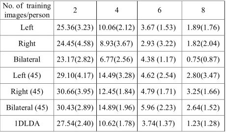
The third experiment is completed on ORL human face dataset. ORL dataset contains forty classes. There are 10 samples per class. All image samples have the resolution of 112×_{96 pixels. For the computational efficiency, here} samples are resized to 56×_{48 pixels. We random select} the training samples and the left samples treated as test samples.

After samples are rotated to the 45_{direction which are}

illustrated in Fig 2, the experiment is done again. In this case, the samples are enlarged to 74×_{74 pixels in order to} keep the original samples not changed and the blank part of every sample is filled with 255(white).

Figure 2. Illustrations of some rotated face images in ORL database.

TABLE IV.

AVERAGE MISCLASSIFICATION RATES(%)USING 2DLDA ON ORIGINAL SAMPLES AND THE ROTATED SAMPLES

No. of training

images/person 2 4 6 8

Left 25.36(3.23) 10.06(2.12) 3.67 (1.53) 1.89(1.76) Right 24.45(4.58) 8.93(3.67) 2.93 (3.22) 1.82(2.04) Bilateral 23.17(2.82) 6.77(2.56) 4.38 (1.17) 0.75(0.87) Left (45) 29.10(4.17) 14.49(3.28) 4.62 (2.54) 2.80(3.47) Right (45) 30.66(3.95) 12.45(1.84) 4.79 (1.71) 3.25(1.66) Bilateral (45) 30.43(2.89) 14.89(1.96) 5.96 (2.23) 2.64(1.52) 1DLDA 27.54(2.40) 10.62(1.78) 3.74(1.37) 1.23(1.28)

Ⅴ_. CONCLUTIONS

In this paper, we discuss the differences between traditional vector-based LDA and matrix-based 2DLDA. It is found that the discriminant power of LDA is always larger than that of 2DLDA. Furthermore, we try to answer the question why 2DLDA outperforms LDA sometimes and we think the main reasons accounting for it are the difference of the stability under nonsingular linear transformation and the power of linear operation between LDA and 2DLDA.Experimental results show that when discriminant information is mainly located along the row/column direction the performance of 2DLDA is superior to that of LDA.

ACKNOWLEDGMENT

This work is supported by National Science Foundation of China under grant No 50875265,50474052.

REFERENCES

[1] P.N. Belhumeur, J. Hespanda, D. Kriegeman, “Eigenfaces

vs Fisherfaces: Recognition using class specific linear

projection,” IEEE Trans. Pattern Anal. Mach. Intell.

London, vol. 19, pp. 711-720, August 1997.

[2] H. Cevikalp, M. Neamtu, M. Wilkes, A. Barkana,

“Discriminative common vectors for face recognition,”

IEEE Trans. Pattern Anal. Mach. Intell.London, vol. 27,

pp. 4-13, September 2005.

[3] L. Chen, H. Liao, M. Ko, J. Lin, G. Yu, “A new LDA based

face recognition system which can solve the small sample

size problem,”Pattern Recognition. London, vol. 33, pp.

1713-1726, December 2000.

[4] R. Huang, Q.S. Liu, H.Q. Lu, S.D. Ma, “Solving the small

sample size problem of LDA,”in: ICPR. , vol. 3, pp. 29-32,

2002.

[5] J. Lu, K.N. Plataniotis, A.N. Venetsanopoulos,

“Regularization studies of linear discriminant analysis in

small sample size scenarios with application to face

recognition,”Pattern Recognition Letters. London, vol. 26,

pp. 181-191, January 2005.

[6] D.Q. Dai, P.C. Yuen, “Regularized discriminant analysis

and its application to face recognition,” Pattern

Recognition. London, vol. 36, pp. 845-847, March 2003.

[7] W. Zhao, R. Chellappa, P.J. Phillips, “Subspace linear

discriminant analysis for face recognition,” Technical

Report CAR- TR-914, CS-TR-4009, University of Maryland, College Park, MD.

[8] P. Zhang, J. Peng , N. Riedel, “Discriminant analysis: a

least squares approximation view,” in: CVPR, pp. 46-46,

2005.

[9] J. Yang, J.Y. Yang, “From image vector to matrix: a

straightforward image projection technique—IMPCA vs.

PCA,” Pattern Recognition. vol. 35, pp. 1997-1999,

September 2002.

[10]J. Yang, D. Zhang, A.F. Frangi, J.Y. Yang, “

Two-dimensional PCA: a new approach to appearance-based

face representation and recognition,”IEEE Trans. Pattern

Anal. Mach. Intell. vol. 26, pp. 131-137, 2004.

[11]M. Li, B. Yuan, “2D-LDA: a novel statistical linear

discriminant analysis for image matrix,” Pattern

Recognition Letter. vol. 26, pp. 527-532, 2005.

[12]H. Kong, L. Wang, E. Teoh, J. Wang, V. Ronda,

“Generalized 2D principal component analysis,”in: IEEE

Conference on IJCNN. Canada, vol. 1, pp. 108-113, 2005.

[13]H. Xiong, M.N.S Swamy, M.O. Ahmad, “Two-dimensional

FLD for face recognition,” Pattern Recognition. vol. 38,

pp. 1121-1124, July 2005.

[14]J. Ye, R. Janardan, Q. Li, “Two-dimensional linear

discriminant analysis,”in: NIPS. 2004.

[15]S. Noushatha, Hemantha, G. Kumar, P. Shivakumara,

“(2D)2 _{LDA: an efficient approach for face recognition,”}

Pattern Recognition. vol. 39, pp. 1396-1400, July 2006.

[16]S.B. Chen, H.F. Zhao, M. Kong, B. Luo, “2D-LPP: A

two-dimensional extension of locality preserving projections,”

Neurocomputing. vol. 70, pp. 912-921, January 2007.

[17]X. Pan, Q.Q. Ruan, “Palmprint recognition with improved

two-dimensional locality preserving projections,” Image

and Vision Computing. vol. 26, pp. 1261-1268, September

2008.

[18]W.S. Zheng, J.H. Lai, S.Z. Li, “1D-LDA vs.

2D-LDA:When is vector-based linear discriminant analysis

better than matrix-based?,”Pattern Recognition. vol. 41, pp.

2156-2172, July 2008.

[19]Z.Z. Liang, Y.F. Li, Shi P F, “A note on two-dimensional

linear discriminant analysis,” Pattern Recognition Letters,

vol. 29, pp. 2122-2128, December 2008.

[20]G.S. Wang, X. Wu, Z. Jia, “Matrix Inequality”,

www.sciencep.com, in press.

[21]ORL, The ORL face database at the AT&T (Olivetti)

research laboratory, 1992.

[22]J.P. Ye, R. Janardan, Q. Li, Park H. “Feature reduction via

generalized uncorrelated linear discriminant analysis,”

IEEE Trans. Knowledge and Data Engineering. vol. 18, pp.

1312-1322, 2006.

Bo Yang was born in Yueyang, China on 22 October 1974.

He is a teacher at Hunan Institute of Science and Technology, China. At the same time, he is working for his Ph.D. in the College of Mechanical and Electrical Engineering, Central South University, China. His current research relates to Sonar signal processing, pattern recognition.

Yingyong Bu is a professor in the College of Mechanical