An Efficient Dimensionality Reduction Approach for Small-sample Size and High-dimensional Data Modeling

An Efficient Dimensionality Reduction Approach

for Small-sample Size and High-dimensional

Data Modeling

Xintao Qiu and Dongmei Fu

School of Automation and Electrical Engineering, University of Science and Technology Beijing, Beijing, China Email: {friend.here, fdm2003}@163.com

Zhenduo Fu

Research and Development Department, Endress Hauser Shanghai Automation Equipment Co. Ltd, Shanghai, China Email: [email protected]

Abstract—As for massive multidimensional data are being generated in a wide range of emerging applications, this paper introduces two new methods of dimension reduction to conduct small-sample size and high-dimensional data processing and modeling. Through combining the support vector machine (SVM) and recursive feature elimination (RFE), SVM-RFE algorithm is proposed to select features, and further, adding the higher order singular value decomposition (HOSVD) to the feature extraction which involves successfully organizing the data into high order tensor pattern. The validation of simulation experiment data shows that the proposed novel feature selection and feature extraction methods can be effectively applied to the research work for analyzing and modeling the data of atmospheric corrosion. The feature selection method pledges that the remaining feature subset is optimal; feature extraction method reserves the original structure, discriminate information, and the integrity of data, etc. Finally, this paper proposes a complete data dimensionality reduction solution that can effectively solve the high-dimensional small sample data problem, and code programming for this solution has been implemented.

Index Terms—feature selection, feature extraction, dimensionality reduction, small-sample data, atmospheric corrosion prediction

I. INTRODUCTION

With the rapid development of technology and applications in data collection and storage capabilities, datasets contain very large feature sets, which brings many difficulties to the work of data analysis and modeling[1, 2]. In recent years, many theories and methods have been used in the data processing and modeling work, such as statistical analysis theory[3], linear regression method[4], neural networks[5]and wavelet analysis theory[6], which have achieved good results and basically met the requirements of engineering. However, with the increasing requirements on the study of the data modeling and practical application, the data

processing and modeling method exposed some deficiency in theory. In fact, with a certain learning machine and a fixed number of training samples, the predictive power reduces as the dimensionality increases, which is called the Hughes effect[7] or Hughes phenomenon[8]. The excessive dimension of the data space often brings the learning algorithms into dimensionality dilemma. So dimensionality reduction is very important for the modeling of small-sample size and high-dimensional data.

Till now, there have been many methods and algorithms for dimensionality reduction in different research fields. Dimensionality reduction theories and methods for small sample data commonly used include Relief algorithm[9], subset search algorithms[10], principal component analysis[11], discriminant analysis[12], canonical correlation analysis[13], partial least squares[14] and manifold learning[15]. Previous analyses of small sample data have not considered combining feature selection process and modeling process yet, and those analyses are based on vector learning that would ignore the changes in each dimension of data[16], which may lead to lose potentially much more compact or useful representations obtained in the original form.

The traditional analytical methods are not a very good solution to solve the curse of dimensionality dilemma caused by the high dimensionality. When the small-sample modeling problem is taken into consideration, we introduce two new methods of dimension reduction to conduct data processing and modeling. First, through combining the support vector machine(SVM) and recursive feature elimination(RFE), SVM-RFE algorithm is proposed to select features in corrosion data, and further, adding the higher order singular value decomposition (HOSVD) to the feature extraction which involves successfully organized the corrosion data into high order tensor pattern. Experimental results shows that the proposed feature selection and feature extraction method can be effectively used in analysis work and data modeling in atmospheric corrosion of metals. The

presented approach is achieving a efficient dimension reduction of processing and modeling, providing a new highly accurate method of small-sample and high-dimensional data processing and modeling.

This paper is organized as follows. Section II focuses on small-sample and high-dimensional data, proposes two dimension reduction algorithms. In Section III, we introduce the data source of our experiment. Then the experiment process and result are described in this section. Section IV discusses the experiment result. A new dimensionality reduction solution for small-sample data and high-dimensional problem is also discussed. Finally, Section V summarizes the major conclusion of this work.

II. METHODS

A. Feature Selection

The target of feature selection is to find a good feature subset to build the model. Dealing with small-sample data modeling problems, the first step is to preprocess data - the linear system or an approximate linear system for example. With a relative error, the linear function f

could be described as the following equation:

( ) ,

f x =〈ω x〉+b with ω∈ Χ ∈,b R, (1)

where ,〈_{⋅ ⋅}〉 denotes the inner product inΧ. The object of equation (1) is to seek a smallerω . Therefore, this problem can be transferred to optimization problem:

ε

ω

ε

ω

ω

≤

−

+

>

<

≤

−

>

<

−

i i

i i

y

b

x

b

x

y

t

s

,

,

.

.

2

1

min

2

(2)

In equation (2), which minimizes the J =(1/ 2)ω 2,

2

( )ωi can be a useful feature ranking criterion when one

feature is removed from the objective function once a time, but when using to remove several features at one time, it will become unreliable. For this reason, Guyon [17] proposed an iterative procedure (Recursive Feature Elimination) to overcome this issue in classification problems. Thus, this method was improved in this paper and applied to small-sample data problem.

This iterative procedure is an instance of backward feature elimination which produces a feature subset ranking opposed to a feature ranking. Feature subsets are nested F1⊂F2 ⊂"⊂F. The point to be noticed is that

the top ranked features may not be the most relevant or necessarily individually. They are chosen to form the subset just because they are optimal when they are put together.

The proposed SVM-RFE algorithm in this paper uses the weight magnitude obtained by SVM as ranking criterion. In order to apply the algorithm to the regression problem, the algorithm SVM-RFE is proposed:

Given a training samples T

l

k x

x x x

X₀ =[ ₁, _2," ," ]

and

[

]

T

1, ,2 k, l

y y y y

= … …

y .

Step1Initialize: Subset of surviving features

[

1,2, n

]

s= … , feature ranked list r=

[ ]

.

Step2 Restrict training samples to good feature indices

)

(:,

0

s

X

X

=

, train the regression

α

_i

−

α

_i*

=

SVM

−

)

,

(

X

y

train

model, compute the weight vector of

dimension length(s)

ω

=

∑

_k

a

k

y

k

x

k.

Step3 Compute the ranking criteria ci =( )ωi 2, for all i.

Step4 Find the feature with the smallest ranking criterion, f =argmin( )c , update feature ranked list

[

s(f ),

]

=

r r .

Step5 Eliminate the feature with smallest ranking criterion s=s(1: f 1,f 1: length( ))− + s .

Step6 If

s

≠

[]

, go to step 2. Step7 Output Feature ranked list r.

B. Feature Extraction

In this section, data was used to organizing into high order tensor pattern. For example, in atmospheric corrosion problem, year and environment influential factors was used to represent two degrees of freedom in a tensor. Comparatively, other linear subspace learning method unfolded the data into a vector, leading to these degrees of freedom that are lost and much of the information in the data tensor might also be lost[18]. There are many applications of HOSVD and higher-order tensor decompositions in the digital image processing and signal filtering[19]. However, the application of HOSVD to atmospheric corrosion data is firstly realized in this paper.

In order to explain HOSVD and higher-order tensor decompositions, the basic multilinear algebra concepts need to be briefly explained in this section.

An

N

th-order tensor is denoted as

_A

∈

_R

I1×I2×"×IN_.

The

n

-mode of

A

is

i

_n

,

n

=

1

,

"

N

. The inner product

of two tensors

_A

,

_B

∈

_R

I1×I2×"×IN _{is defined as}

∑ ∑

= =

∑

=

⋅

>=

<

1

1 2

2 1 1 2 1 2

1 1 , , , ,

,

I

i I i

I

i i i i i

N

n N N

B

A

B

A

"

_{" "}

and the Frobenius norm of

A

is defined as

>

<

=

A

A

A

_F

,

. The “

n

-mode vectors” of

A

are

defined as the

I

n- dimensional vectors obtained from

A

by varying the index

i

n while keeping all the other indices fixed[18]. Unfolding

A

along the

m

-mode is

denoted as _{( )} Im (I1 Im1 Im1 IN)

m

× × × × ×

× − +

∈

" "

R

A

. The column

vectors of

A

₍m₎ are the

m

-mode vectors of

A

. The

d

-mode product

A

×

_d

U

, is a tensor with matrix

∑

⋅

=

×

_{− +}

d n n d

n d n

d j i i i i i j i

i i

d

A

A

)

(

)

0 2 4 6 8 10 12 0

2 4 6 8 10

12 Relative errors of test data

Recursion times (number of removed features)

A

bso

lute

v

alue

o

f re

la

tiv

e e

rror(%

) The sixth yearThe sixteeenth year

Figure 1. Modeling comparison of HOSVD and PCA.

From multilinear algebra[20], tensor

A

can be

decomposition as the product

) ( )

2 ( 2 ) 1 (

1 N N

S

A

=

×

U

×

U

×

"

×

U

(3)

where T T _NT

N

A

S

=

×

₁

U

(1)

×

₂

U

(2)

×

"

×

U

( ) is

core tensor and ( )

(

₁( ) (₂) (n)

)

I n n n

n

u

u

u

U

=

"

is an

orthogonal matrix. The Higher-order tensor decomposition algorithm[21] is a form of higher-order principal component analysis. It decomposes a tensor into a core tensor multiplied (or transformed) by a matrix along each mode.

Higher-order tensor decomposition algorithm Given a tensor,

_A

∈

_R

I1×I2×"×IN

Step1 Initialize

_U

(n)

∈

_R

In×R for

_i

_n

_N

n

,

=

,1

"

, let R

I

n _n

R

×

∈

) ( 0

U

be leading left singular vectors of

A

₍n₎.

Setp2 For

t

=

0

1,

,

"

,

T

_max

- For

n

=

0

,

,1

L

,

N

* Calculate

=

×

×

T

×

"

t

T t

A

y

₁

U

(1) ₂

U

(2)

T N t N T

n t n T n t n

) ( )

1 ( 1 ) 1 (

1

U

×

U

×

×

U

×

+

+ −

−

"

* Set (n) t

U

be leading left singular vectors of

) (n

y

- if

y

_F

−

A

_F

<

_η

, break go step3.

Step3 Let

{

U

}

=

{

U

_K

}

, where

K

is the index of the

final result of step2.

Step4 Set

y

=

A

×

{

U

T

}

.

III. EXPERIMENT AND RESULT

A. Data Source and Raw Data

The experiment data are chosen from the website ‘China Gateway to Corrosion & Protection’. In this paper, the corrosion data of A3 steel during ten years and the relevant environmental factors in Guangzhou test station was selected[22], which is listed below in Table 1: B. SVM-RFE

In this model, Support Vector Regression (SVR) method was used as the regression strategy after SVM-RFE. The samples of the sixth year and the sixteenth year were randomly chosen to act as test data here, and the other eight sets of samples were served as training data.

The programmer was built based on LIBSVM toolbox coded by Chih-Chung Chang and Chih-Jen Lin[23]. Experiment parameters were set as follows: The cost parameter C=1000, the ε in loss function ε=1.5 10× −6.

Fig. 1 shows the absolute value of relative error of the test data, towards the models after every recursions[24].

The elimination sequence is: Temperature, precipitation, sunshine hours, HCl, SO3, SO2, H2S, relative humidity,

Cl-_{, NH}

3, NO2. It was found that before SVM-RFE, even

SVR is used for regression, the relative errors are quite large — about 10% and 7%. After the forth and fifth recursion, the error lines drop rapidly. It demonstrates that the first removed four or five factors are unrelated or redundant ones in this corrosion model. After these features eliminated, the test errors decrease to a quite low level.

1 2 3 4 5 6 7 8 9 10 0.1

0.12 0.14 0.16 0.18 0.2

0.22 The modeling comparison

Testing year

Co

rr

os

ion am

ount

(m

m

)

real corrosion amount tensor decomposition principal component analysis

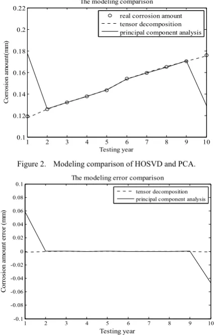
Figure 2. Modeling comparison of HOSVD and PCA.

1 2 3 4 5 6 7 8 9 10

-0.1 -0.08 -0.06 -0.04 -0.02 0 0.02 0.04 0.06 0.08

0.1 The modeling error comparison

Testing year

Corros

ion

am

ou

nt er

ro

r (m

m

)

tensor decomposition principal component analysis

Figure 3. The modeling error comparison of HOSVD and PCA.

C. HOSVD

In this model, the normalization of data was first conducted, and then the tensor decomposition and principal component analysis were employed to reduce the dimensionality of the data, at last the same modeling approach was used to data modeling. In the modeling process, data from the sixth year and the sixteenth year was randomly chosen as testing data, the other eight sets of samples were served as training data.

Our algorithm programmer is built based on MATLAB Tensor Toolbox Version 2.5 coded by Brett W. Bader, Tamara G. Kolda[21]. In the tensor decomposition, we use the tucker tensor decomposition algorithm, and set the maximum number of iterations 50, the training stop error

1

×

10

−4 , the experiment parameters are as follows: The cost parameter C=1000, the

ε

in loss function

4

10

2

_×

−

=

ε

.

The comparative results of tensor decomposition and principal components analysis modeling are listed in Fig.2 and 3. From these figures, it can be seen that with the same modeling approach, the data extraction by tensor decomposition can achieve better modeling and prediction effect. At the same time, when using HOSVD algorithm, even threshold value

ε

of loss function in support vector machine (the threshold

ε

bigger the support vector less) is bigger than the SVM-RFE algorithm, it can still achieve better modeling result.

IV. DISCUSSION

Through the experiment and simulation, it was proven that the proposed SVM-RFE and HOSVD dimensionality reduction methods had better performance than existing methods in dealing with atmospheric corrosion prediction. At the same time, the proposed method is not only suitable for corrosion data, but can also be used for other high-dimensional data. In the practical application, a dimensionality reduction solution for high-dimensional small sample data analysis can be proposed:

First, feature selection. If the original factors/attribute of data need keeping, the feature selection method could be used. It can provide an optimal feature subset while keeping all the physical meaning of the original factors/attribute.

Second, feature extraction. If feature selection is unable to meet the requirements of the modeling, or you are more concerned about the independence and non-correlation of the data after dimensionality reduction, use the feature extraction method.

Third, regression or fitting. This process is a loop cycle process. Different methods and algorithms can be selected to deal with different projects. If the predictive power of the learning machine fails to meet the requirements of modeling after optimize the learning machine, the loop returns to the first step and change the dimensionality reduction method.

V. CONCLUSIONS

The work in this paper is based on the achieved experimental data. Under the consideration of the small sample data with high dimension, this paper proposes a dimensionality reduction solution for this kind of data. Overall, the proposed data dimensionality methods have the following advantages over previous methods:

1)A compact dimensionality reduction solution for high-dimensional small sample data analysis was proposed. The SVM-RFE algorithm can keep the original factors/attribute of data and ensures the remaining feature subset optimal after the removal of the corresponding attributes. The application of tensor decomposition to the dimensionality reduction of material corrosion data was innovative for this work. During the dimension reduction process, the changes of data in each dimension can be considered, and the original structure and discriminate information of data can be kept to the maximum extent, which guarantee the integrity of data.

2)Simulation experiment data validation shows that the proposed SVM-RFE feature selection method can keep the original factors/attribute of the data in atmospheric corrosion of metals and ensure that the remaining feature subset is optimal for modeling. The dimensionality reduction method based on HOSVD can consider the changes of dimension in year and environmental factors, keeps the original structure of the atmospheric corrosion data, and has better performance than existing methods.

corrosion data in seawater, soil corrosion data and so on. Meanwhile, the processing can be treated as a reference to deal with other small sample with high-dimensional data.

ACKNOWLEDGMENT

This research was supported by National Nature Science Foundation of China (No.51131001) and Beijing Key Discipline Development Program of Beijing Municipal Commission of Education (No.XK100080537).

The authors are also grateful to

Brett W. Bader, Tamara G. Kolda and others. MATLAB Tensor Toolbox Version 2.5, Available online, January 2012.

URL: http://www.sandia.gov/~tgkolda/TensorToolbox/ Chih-Chung Chang and Chih-Jen Lin who made their LIBSVM source code available through the Internet .

URL:http://www.csie.ntu.edu.tw/~cjlin/libsvm

REFERENCES

[1] J. Long, X. Shen, and H. Chen, "A robust thresholding algorithm framework based on reconstruction and dimensionality reduction of the three dimensional

histogram," Journal of Computers (Finland), vol. 8, pp.

645-652, 2013.

[2] Z. Wang and X. Sun, "Image retrieval with tensor biased

discriminant embedding," Journal of Computers (Finland),

vol. 8, pp. 1207-1213, 2013.

[3] M. K. Cavanaugh, R. G. Buchheit, and N. Birbilis, "Modeling the environmental dependence of pit growth

using neural network approaches," Corrosion Science, vol.

52, pp. 3070-3077, Sep 2010.

[4] H. Lu, H. Liyan, and Z. Hongwei, "Credit scoring model hybridizing artificial intelligence with logistic regression," Journal of Networks, vol. 8, pp. 253-261, 2013.

[5] J. Li, S. Hong, S. Xia, and S. Luo, "Neural network based

popularity prediction for IPTV system," Journal of

Networks, vol. 7, pp. 2051-2056, 2012.

[6] W. Sun, H. Wang, and D. Qian, "A novel error resilient scheme for waveletbased image coding over packet

networks," Journal of Networks, vol. 7, pp. 1046-1053,

2012.

[7] T. Oommen, D. Misra, N. K. C. Twarakavi, A. Prakash, B. Sahoo, and S. Bandopadhyay, "An objective analysis of Support Vector Machine based classification for remote

sensing," Mathematical Geosciences, vol. 40, pp. 409-424,

May 2008.

[8] G. Hughes, "On the mean accuracy of statistical pattern

recognizers," Information Theory, IEEE Transactions on,

vol. 14, pp. 55-63, 1968.

[9] L. P. Wang, N. N. Zhou, and F. Chu, "A general wrapper

approach to selection of class-dependent features," Ieee

Transactions on Neural Networks, vol. 19, pp. 1267-1278, Jul 2008.

[10] M. Kudo and J. Sklansky, "Comparison of algorithms that

select features for pattern classifiers," Pattern Recognition,

vol. 33, pp. 25-41, Jan 2000.

[11] M. Thameri, K. Abed-Meraim, and A. Belouchrani, "Low complexity adaptive algorithms for Principal and Minor

Component Analysis," Digital Signal Processing, vol. 23,

pp. 19-29, Jan 2013.

[12] B. Xu, K. Z. Huang, and C. L. Liu, "Maxi-Min

discriminant analysis via online learning," Neural

Networks, vol. 34, pp. 56-64, Oct 2012.

[13] D. R. Hardoon, S. Szedmak, and J. Shawe-Taylor, "Canonical correlation analysis: An overview with

application to learning methods," Neural Computation, vol.

16, pp. 2639-2664, Dec 2004.

[14] P. P. Roy and K. Roy, "On some aspects of variable

selection for partial least squares regression models," Qsar

& Combinatorial Science, vol. 27, pp. 302-313, Mar 2008. [15] M. Belkin, P. Niyogi, and V. Sindhwani, "Manifold

regularization: A geometric framework for learning from

labeled and unlabeled examples," Journal of Machine

Learning Research, vol. 7, pp. 2399-2434, Nov 2006. [16] H. Lu, N. P. Konstantinos, and A. N. Venetsanopoulos,

"MPCA: Multilinear principal component analysis of

tensor objects," IEEE Transactions on Neural Networks,

vol. 19, pp. 18-39, Jan 2008.

[17] I. Guyon, J. Weston, S. Barnhill, and V. Vapnik, "Gene selection for cancer classification using support vector

machines," Machine Learning, vol. 46, pp. 389-422, 2002.

[18] H. Lu, K. N. Plataniotis, and A. N. Venetsanopoulos, "A survey of multilinear subspace learning for tensor data," Pattern Recognition, vol. 44, pp. 1540-1551, Jul 2011. [19] T. G. Kolda and B. W. Bader, "Tensor Decompositions

and Applications," Siam Review, vol. 51, pp. 455-500, Sep

2009.

[20] L. De Lathauwer and J. Vandewalle, "Dimensionality reduction in higher-order signal processing and rank-(R-1,

R-2, ..., R-N) reduction in multilinear algebra," Linear

Algebra and Its Applications, vol. 391, pp. 31-55, Nov 2004.

[21] W. B. Brett and G. K. Tamara, "Algorithm 862: MATLAB

tensor classes for fast algorithm prototyping," ACM Trans.

Math. Softw., vol. 32, pp. 635-653, 2006.

[22] F. Zhenduo, F. Dongmei, and L. Xiaogang, "Atmospheric Corrosion Modelling with SVM Based Feature Selection," presented at the Computational Intelligence and Software Engineering, 2009. CiSE 2009. International Conference on, 2009.

[23] C. Chih-Chung and L. Chih-Jen, "LIBSVM: A library for

support vector machines," ACM Trans. Intell. Syst.

Technol., vol. 2, pp. 1-27, 2011.

[24] X. T. Qiu, D. M. Fu, Z. D. Fu, K. Riha, and R. Burget, "The Method for Material Corrosion Modelling And Feature Selection with SVM-RFE," presented at the 34th International Conference on Telecommunications and Signal Processing, 2011.

Xintao Qiu is currently working toward the Ph.D. degree in School of Automation and Electrical Engineering with University of Science and Technology Beijing. His research interests are in the areas of wireless sensor network and data mining. P.R. China (e-mail: [email protected]).

Dongmei Fu is Professor and Co-Chair of the School of Automation and Electrical Engineering at University of Science and Technology Beijing. P.R. China (e-mail: [email protected]).