Essays in Asset Pricing

University of Pennsylvania

ScholarlyCommons

Publicly Accessible Penn Dissertations

1-1-2015

Essays in Asset Pricing

Darien Huang

University of Pennsylvania, darien.huang@gmail.com

Follow this and additional works at:

http://repository.upenn.edu/edissertations

Essays in Asset Pricing

Abstract

In the first chapter ``Gold, Platinum, and Expected Stock Returns'', I show that the ratio of gold to platinum prices (GP) reveals variation in risk and proxies for an important economic state variable. GP predicts future stock returns in the time-series and explains variation in average stock returns in the cross-section. GP outperforms existing predictors and similar patterns are found in international markets. GP is persistent and significantly correlated with option-implied tail risk measures. An equilibrium model featuring recursive preferences, time-varying tail risk, and shocks to preferences for gold and platinum can account for the asset pricing dynamics of equity, gold, and platinum markets, and quantitatively explain the return predictability. In the second chapter ``Risk Adjustment and the Temporal Resolution of Uncertainty: Evidence from Options Markets'', we examine risk-neutral probabilities, which are observable from option prices and combine objective probabilities and risk adjustments across economic states. We consider a recursive-utility framework to separately identify objective probabilities and risk adjustments using only observed market prices. We find that a preference for early resolution of uncertainty is important in explaining the cross-section of risk-neutral and objective probabilities in the data. Failure to incorporate a preference for the timing of the resolution of uncertainty (e.g., expected utility models) can significantly overstate the implied probability of, and understate risk compensations for, adverse economic states. In the third chapter ``Volatility-of-Volatility Risk'', we show that time-varying volatility of volatility is a significant risk factor which affects the cross-section and time-series of index and VIX option returns, beyond volatility risk itself. Volatility and volatility-of-volatility movements are identified from index and VIX option prices, and correspond to the VIX and VVIX indices in the data. Delta-hedged returns for index and VIX options are negative on average, and more negative for strategies more exposed to volatility and volatility-of-volatility risks. In the time-series, volatility and volatility of volatility significantly predict delta-hedged returns with a negative sign. The evidence is consistent with a no-arbitrage model featuring time-varying volatility and volatility-of-volatility factors which are negatively priced by investors.

Degree Type Dissertation

Degree Name

Doctor of Philosophy (PhD)

Graduate Group Finance

First Advisor Amir Yaron

Subject Categories

ESSAYS IN ASSET PRICING

Darien Huang

A DISSERTATION

in

Finance

For the Graduate Group in Managerial Science and Applied Economics

Presented to the Faculties of the University of Pennsylvania

in

Partial Fulfillment of the Requirements for the

Degree of Doctor of Philosophy

2015

Supervisor of Dissertation

Amir Yaron, Robert Morris Professor of Banking and Finance

Graduate Group Chairperson

ACKNOWLEDGEMENT

I would like to thank my advisors Franklin Allen, Ivan Shaliastovich, and Amir Yaron

(Chair) for their help, support, and guidance. I also thank Andy Abel, Erik Gilje, Itay

Goldstein, Mete Kilic, Nick Roussanov, Luke Taylor, Rob Stambaugh, and Jessica Wachter

ABSTRACT

ESSAYS IN ASSET PRICING

Darien Huang

Amir Yaron

In the first chapter “Gold, Platinum, and Expected Stock Returns”, I show that the ratio of

gold to platinum prices (GP) reveals variation in risk and proxies for an important economic

state variable. GP predicts future stock returns in the time-series and explains variation in

average stock returns in the cross-section. GP outperforms existing predictors and similar

patterns are found in international markets. GP is persistent and significantly correlated

with option-implied tail risk measures. An equilibrium model featuring recursive

prefer-ences, time-varying tail risk, and shocks to preferences for gold and platinum can account

for the asset pricing dynamics of equity, gold, and platinum markets, and quantitatively

explain the return predictability.

In the second chapter “Risk Adjustment and the Temporal Resolution of Uncertainty:

Ev-idence from Options Markets”, we examine risk-neutral probabilities, which are observable

from option prices and combine objective probabilities and risk adjustments across economic

states. We consider a recursive-utility framework to separately identify objective

probabil-ities and risk adjustments using only observed market prices. We find that a preference for

early resolution of uncertainty is important in explaining the cross-section of risk-neutral

and objective probabilities in the data. Failure to incorporate a preference for the timing of

the resolution of uncertainty (e.g., expected utility models) can significantly overstate the

implied probability of, and understate risk compensations for, adverse economic states.

In the third chapter “Volatility-of-Volatility Risk”, we show that time-varying volatility of

volatility is a significant risk factor which affects the cross-section and time-series of index

movements are identified from index and VIX option prices, and correspond to the VIX and

VVIX indices in the data. Delta-hedged returns for index and VIX options are negative

on average, and more negative for strategies more exposed to volatility and

volatility-of-volatility risks. In the time-series, volatility-of-volatility and volatility-of-volatility of volatility-of-volatility significantly predict

delta-hedged returns with a negative sign. The evidence is consistent with a no-arbitrage

model featuring time-varying volatility and volatility-of-volatility factors which are

TABLE OF CONTENTS

ACKNOWLEDGEMENT . . . iii

ABSTRACT . . . iv

LIST OF TABLES . . . ix

LIST OF ILLUSTRATIONS . . . x

CHAPTER 1 : Gold, Platinum, and Expected Stock Returns . . . 1

1.1 Introduction . . . 1

1.2 Empirical Results . . . 5

1.3 Gold and Platinum Markets . . . 15

1.4 Economic Model . . . 19

1.5 Calibration and Model Simulation Results . . . 29

1.6 Conclusion . . . 32

CHAPTER 2 : Risk Adjustment and the Temporal Resolution of Uncertainty . . . 56

2.1 Introduction . . . 56

2.2 Theoretical Framework . . . 61

2.3 Economic Model . . . 69

2.4 Empirical Analysis . . . 77

2.5 Robustness . . . 85

2.6 Conclusion . . . 88

CHAPTER 3 : Volatility-of-Volatility Risk . . . 100

3.1 Introduction . . . 100

3.2 Model . . . 105

3.4 Evidence from Options . . . 117

3.5 Robustness . . . 123

3.6 Conclusion . . . 126

APPENDIX . . . 138

A.1 Appendix for Gold, Platinum, and Expected Stock Returns . . . 138

A.2 Appendix for Risk Adjustment and the Temporal Resolution of Uncertainty 150 A.3 Appendix for Volatility-of-Volatility Risk . . . 152

LIST OF TABLES

TABLE 1.1 : Summary Statistics for Predictors . . . 33

TABLE 1.2 : U.S. Stock Return Predictability . . . 34

TABLE 1.3 : Univariate Return Predictability . . . 34

TABLE 1.4 : Bivariate Return Predictability: Short Horizon . . . 35

TABLE 1.5 : Bivariate Return Predictability: Long Horizon . . . 36

TABLE 1.6 : Out-of-Sample Tests . . . 37

TABLE 1.7 : International Markets Return Predictability . . . 38

TABLE 1.8 : Predicting Dividend Growth . . . 39

TABLE 1.9 : Cross-Sectional Implications . . . 40

TABLE 1.10 : GP and Tail Risk . . . 41

TABLE 1.11 : Inventory Financing for Jewellers . . . 42

TABLE 1.12 : Gold and Platinum Returns . . . 42

TABLE 1.13 : Model Parameters . . . 43

TABLE 1.14 : Simulation Results: Asset Pricing Moments . . . 44

TABLE 1.15 : Simulation Results: Return Predictability . . . 45

TABLE 1.16 : Gold and Platinum Supply Dynamics . . . 46

TABLE 2.1 : Model Calibration . . . 90

TABLE 2.2 : Model Output . . . 91

TABLE 2.3 : Economic Variables in Aggregate States . . . 91

TABLE 2.4 : Implications for Probabilities and Risk Compensations . . . 92

TABLE 3.1 : Summary Statistics . . . 128

TABLE 3.2 : Predictability of Realized Measures . . . 129

TABLE 3.3 : Delta-Hedged Option Gains . . . 130

TABLE 3.5 : Predictability of Delta-Hedged SPX Option Gains . . . 132

TABLE 3.6 : Predictability of Realized Measures - Alternate Specifications . . . 133

LIST OF ILLUSTRATIONS

FIGURE 1.1 : Gold and Platinum Prices . . . 47

FIGURE 1.2 : Log GP Ratio . . . 48

FIGURE 1.3 : Rolling Regressions - GP ratio . . . 49

FIGURE 1.4 : Rolling Regressions - PD ratio . . . 50

FIGURE 1.5 : Cross-Sectional Pricing . . . 51

FIGURE 1.6 : Gold and Platinum Demand . . . 52

FIGURE 1.7 : Gold Lease Rates 2007 - 2009 . . . 52

FIGURE 1.8 : Multinomial Disaster Size Distribution . . . 53

FIGURE 1.9 : Per-Capita Gold and Platinum Stock Growth . . . 54

FIGURE 1.10 : Implied Volatility Slope by Disaster Intensities . . . 55

FIGURE 2.1 : Probabilities and Risk Adjustments: Model . . . 93

FIGURE 2.2 : Probabilities and Risk Adjustments: Model, Return States . . . 94

FIGURE 2.3 : Empirical Distribution of Market Capital Gains . . . 95

FIGURE 2.4 : Implied Volatility Curves in Economic States . . . 95

FIGURE 2.5 : Recovered Risk-Neutral Densities in Economic States . . . 96

FIGURE 2.6 : Probabilities and Risk Adjustments: Data . . . 97

FIGURE 2.7 : Implied Bad State Probability . . . 98

FIGURE 2.8 : Implied Probabilities and Risk Adjustments: Monthly Data . . 99

FIGURE 3.1 : Time Series Plot . . . 135

FIGURE 3.2 : Realized Measures . . . 136

FIGURE 3.3 : Vega and Gamma by Moneyness . . . 136

CHAPTER 1 : Gold, Platinum, and Expected Stock Returns

1.1. Introduction

“As gold’s unquenchable beauty shines like the sun, people have turned

to it to protect themselves against the darkness ahead.”

— Bernstein (2012), The Power of Gold: The History of an Obsession

Gold is one of the most important assets in financial markets and the global economy. As the

author Peter Bernstein summarizes above, gold is viewed as two things: it is a consumption

good (mostly jewellery) and it is also seen as something valuable in times of severe distress.

Platinum, on the other hand, is a precious metal with similar uses as gold in consumption.

Therefore, the ratio of gold to platinum prices should be largely insulated from shocks to

consumption and jewelry demand, and should instead reveal variation in risk and proxy for

an important economic state variable. I investigate three questions in this paper.

First, I ask whether the ratio of gold to platinum prices (GP) predicts future stock returns

in the time-series and explains variation in average stock returns in the cross-section. I

show empirically that GP is a strong predictor of future stock returns. A one standard

deviation increase in GP predicts a 6.4% increase in U.S. stock market excess returns over

the following year. GP outperforms nearly all existing return predictors and is robust to

various econometric inference concerns highlighted in the literature. Gold and platinum are

actively traded around the world, and similar patterns of stock return predictability are

found in international markets. GP risk is priced in the cross-section of stock returns and

and NBER recession indicators from 1975 - 2013.2 We see in the data that gold prices fall

in recessions, albeit by less than platinum prices. For example, in the 1981 - 1982 recession,

real gold prices fell 32% peak to trough, and in the recent 2008 - 2009 financial crisis real

gold prices fell 22%. Unlike index put options or VIX futures, gold futures would not have

helped investors hedge downside risks during the crises. Not by coincidence, the real price

of platinum fell by 39% and 59% over the same periods, respectively.

To the extent that investors view shocks to gold prices as short-lived, flight-to-liquidity

phenomena, I find that this is not the case. Shocks to GP do not correlate with shocks to

transient measures of liquidity risk such as the Pastor and Stambaugh (2003) factor, and

instead have a much longer half-life. Furthermore, GP is significantly related to measures

of economic tail risk including the slope of the implied volatility curve for S&P500 index

options, and the Bakshi, Kapadia, and Madan (2003) model-free risk-neutral skewness.3

These findings lead to my final question, which is whether an extension of the time-varying

disaster risk model (Wachter (2013)), which features recursive preferences and stochastic

disaster probabilities, can quantitatively explain the time variation and return predictability

of GP while simultaneously accounting for the asset pricing dynamics of equity, gold, and

platinum markets, without any additional risk factors. The model is motivated by the fact

that, under no arbitrage, investors are indifferent between buying gold or leasing gold in

perpetuity (Barro and Misra (2013)).

I adopt a three-good model where agents derive utility from nondurable consumption as

well as service flows from gold and platinum, which are non-depreciating durable goods

with negligible outlays relative to nondurable consumption. In normal times, service flows

from gold and platinum (which can be thought of as jewellery) complement nondurable

2

I focus exclusively on the post-gold standard era, where gold prices vary freely by a market mechanism. While the “Nixon shock” of 1971 temporarily suspended convertibility of U.S. dollars into gold at $35 per oz, a new peg was later put in place at $38 per troy oz, followed by $42.22. Gold convertibility was only completely abolished by November 1973 (Lannoye (2011)). Executive Order 6102, put in place by President Franklin Roosevelt in 1933, banned gold trading within the United States. This act was repealed by President Gerald Ford in 1974 and took effect on December 31st, 1974. See Public Law 93-373.

3

consumption and are highly procyclical. However, when the probability of a consumption

disaster is high, agents display an increased preference for gold relative to platinum. This is

motivated by historical and institutional reasons, since gold is viewed as financial collateral

and is formally recognized as such by the Basel Accords.4

The countercyclical benefits to physical ownership of gold and platinum are modeled in

reduced-form using a pair of stochastic processes which are proportional to the

probabil-ity of a consumption disaster; gold is calibrated to have greater countercyclical benefits

than platinum, which is both consistent with the historical and institutional facts and also

allows the model to rationalize the low gold lease rate and risk premium observed in the

data.5 In the model, GP is insulated from shocks to consumption since they affect gold

and platinum prices equally. Increases in disaster probabilities raise risk premia, leading to

higher discount rates and lower stock prices. Gold and platinum prices fall as well because

of strong discount rate effects, although gold prices fall by less than platinum prices due to

the higher countercyclical component of its service flow. As a result, GP is high when stock

prices are low and the equity risk premium is high, giving GP the power to predict future

stock market excess returns. The model quantitatively captures the key moments of gold

and platinum returns, while remaining consistent with standard asset pricing moments such

as the equity premium and risk-free rate. This is achieved without introducing additional

state variables, which suggests that gold and platinum returns can largely be explained by

the same risk factors affecting stocks and bonds.

Barro and Misra (2013) study gold returns in a Lucas (1978) endowment economy with rare

consumption disasters. The authors match the low gold risk premium using a high elasticity

rather than substitutable relationship (one cannot wear jewellery in place of consuming food,

but jewellery is highly valued when food is plentiful). Second, optimality conditions reveal

that the elasticity of substitution is inversely proportional to the degree of consumption

leverage. Following analysis similar to Wachter (2013), I show that substitutability results

in the counterfactual prediction that gold lease rates fall (gold prices rise) when disaster

probabilities increase.

This paper contributes to the literature on return predictability by demonstrating that GP,

a model-free measure available in real-time, is robust to and in most cases outperforms

existing forecasting variables including equity valuation ratios (in various forms), the

de-fault spread, term spread, inflation, implied cost of capital, consumption-wealth ratio, and

variance premium.6 The predictive power of GP is stable both out-of-sample and over

sub-samples, which alleviates concerns raised by studies such as Goyal and Welch (2008),

who show that many predictors such as valuation ratios have low forecasting performance

out-of-sample and unstable forecasting ability over sub-samples.

This paper extends the growing literature on gold and gold lease rates. To my knowledge,

Barro and Misra (2013) is the only other paper to value gold in an equilibrium model. Fama

and French (1988) analyze the behavior of metals prices over the business cycle based on the

Brennan (1958) theory of storage. While base metals such as aluminum and copper behave

as the theory of storage predicts, precious metals such as gold seem unresponsive; Fama

and French hypothesize that this is due to low storage costs for precious metals.Tufano

(1996) studies risk management practices in the gold mining industry. Schwartz (1997),

Casassus and Collin-Dufresne (2005), and Le and Zhu (2013) study gold lease rates (known

as “convenience yields” in the commodities literature) using dynamic term structure models.

6

Erb and Harvey (2013) examine various theories regarding gold returns, including whether

gold prices appreciate when stock prices fall. The authors find that many of the largest

S&P500 declines were associated with falling gold prices.

Finally, this paper draws on the literature examining the impact of heavy-tailed shocks

to economic state variables on asset prices. Examples from the option pricing literature

include Bates (2000), Duffie, Pan, and Singleton (2000), Pan (2002), and Broadie, Chernov,

and Johannes (2007). Jurek (2014) discusses the impact of crash risk on currency carry

trade returns. Examples from the general equilibrium literature include the rare disasters

framework (Rietz (1988), Barro (2006), Gabaix (2012), Gourio (2012), Wachter (2013),

Nowotny (2011), Seo and Wachter (2014)), as well as extensions of the Bansal and Yaron

(2004) long-run risks framework incorporating jumps in economic fundamentals (Eraker

and Shaliastovich (2008), Bansal and Shaliastovich (2011), Benzoni, Collin-Dufresne, and

Goldstein (2011), Drechsler and Yaron (2011)).

The paper proceeds as follows; data sources are discussed as the relevant sections are

pre-sented. Section 2 presents the empirical results on stock return predictability, cross-sectional

evidence, and the relationship between GP and tail risk measures. Section 3 discusses key

aspects of gold and platinum markets, focusing on sources of demand for each metal, the

leasing markets, and return dynamics. Section 4 presents the model. Section 5 discusses

the model calibration and simulation results. Section 6 concludes.

1.2. Empirical Results

to this, for platinum prices I use dealer prices from the U.S. Geological Survey.8 The log

GP ratio is calculated as the natural logarithm of the ratio of gold to platinum prices.9 My

measure of U.S. stock returns is the CRSP value-weighted index. The risk-free rate is the

1 month U.S. Treasury bill rate. I compare the performance of GP to various forecasting

variables proposed in the literature.

• Price-Dividend Ratio (logP D) is the log ratio of aggregate stock market price divided

by the sum of the past twelve months of dividends. Dividends are computed from

the difference between the CRSP value-weighted index return including and exluding

dividends.

• Price-Earnings Ratio (logP E) is the cyclically-adjusted log ratio of aggregate stock

market price divided by past earnings, obtained from Robert Shiller’s website.

• Net Payout Ratio (logP N Y) is the log ratio of total market capitalization divided

by the sum of dividends, repurchases, and share issuance, as described in Boudoukh

et al. (2007) and obtained from Michael Roberts’s website. The series is available

until December 2010.

• Implied Cost of Capital (ICC) is rate of return which solves the long horizon dividend

discount model, constructed from I/B/E/S analyst earnings per share forecasts, as

described in Li et al. (2013). The series starts from January 1977.

• Default Spread (DF SP) is the percentage difference in yield between Moody’s Baa

and Aaa rated corporate bonds and obtained from the Federal Reserve Bank of St.

Louis (FRED) website.

• Term Spread (T M SP) is the percentage difference in yield between 10 year U.S.

government bonds and 3 month U.S. Treasury bills and obtained from FRED. 8

My results are nearly unchanged using platinum prices directly obtained from Platts, which is a large data vendor for metals markets.

9

• Inflation (IN F L) is the log growth rate of the Consumer Price Index (All Urban

Consumers: All Items), in percentages, from FRED.

• Consumption-Wealth Ratio (CAY) is the Lettau and Ludvigson (2001) measure of

the consumption-wealth ratio, obtained from Martin Lettau’s website. Monthly

ob-servations are computed by interpolating the quarterly obob-servations. The series is

available until March 2013.

• Variance Premium (V RP) is the difference between model-free implied variance

com-puted from S&P500 option prices (V IX2) and realized variance computed from

5-minute tick data over the past 30 days. The data for the VIX is obtained from the

CBOE website, and the data for realized variance is from Hao Zhou’s website. The

series starts from January 1990.

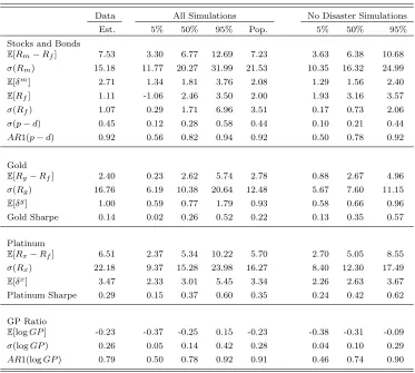
Figure 1.2 plots the time-series of GP (solid line) along with the price-dividend ratio (dashed

line). The average level of GP is below zero; gold trades at a 20% discount to platinum on

average, consistent with platinum being a much scarcer metal. GP is strongly

countercycli-cal and peaks during times of economic and financial distress including all NBER recessions

between 1975 - 2013, as well as the October 1987 stock market crash, 1998 Russian default

and LTCM crisis, and 2011 U.S. debt ceiling crisis. Table 1.1 presents summary statistics

for all the predictors. With the exception of the variance premium and inflation, all other

predictors are quite persistent. The AR(1) coefficient for GP is 0.98, which is inside the

unit circle. Formally, a Dickey and Fuller (1979) stationarity test rejects the null of a unit

root for logGP at the 5% level.10 The high persistence of GP is in contrast to the view

which raises the required yield on their corporate bonds. GP is positively correlated with

ICC since the cost of capital for firms is high in adverse economic conditions. High values

ofCAY are associated with high risk premia, and accordingly we see a positive correlation

of GP with CAY (Lettau and Ludvigson (2001)). GP is not correlated withIN F L; this is

expected, since inflation equally affects both the numerator and denominator of the ratio.

1.2.2. Stock Return Predictability

My measure of U.S. stock returns is the CRSP value-weighted index. The risk-free rate is

the 1 month U.S. Treasury bill rate. I compare the performance of GP to various forecasting

variables proposed in the literature. Table 1.2 shows the main predictability result of the

paper. I run the regression:

12 h

h

X

i=1

logRt+i−logRft+i=β0+β1logGPt+t+h (1.1)

Long-horizon returns are constructed from overlapping monthly returns. The top panel

uses ordinary least squares regression with Newey and West (1987) HAC robust standard

errors.11 At the 1 month horizon, the degree of predictability is fairly low with an R2 just

above 1%; however, the estimated slope is statistically significant with a 2.82 t-statistic.

We see similar patterns of predictability up to the 1 year horizon, which has an R2 of

16.57%. The bottom panel uses the vector autoregression (VAR) framework as in Hodrick

(1992), which is potentially more conservative for overlapping returns, although it imposes

parametric assumptions. The point estimates are very similar, although theR2 is lower (yet

still very large at 10.89% for the 1 year horizon) using the VAR. For longer horizons of 2 to

5 years, the estimated coefficients are still significant although the magnitude is decreasing.

The estimated coefficient on logGP for the one year horizon is 0.243, the standard deviation

of logGP is 0.266, so a one standard deviation increase in logGP is associated with a 6.4%

increase in U.S. stock market excess returns over the following year. For all horizons from 11

1 month to 5 years, the estimated slopes are statistically significant.

Table 1.3 shows the results of univariate predictability regressions for each of the

predic-tors. For short horizon returns (1 and 3 months), only GP, and V RP are statistically

significant at conventional levels, withICC significant at the 10% level. At the

intermedi-ate 1 year horizon, GP, ICC, andV RP are strongly significant, while T M SP and IN F L

are marginally significant. At this frequency, GP has the highest R2 _{of all predictors. For}

long horizon (e.g. 5 year) returns, GP is still significant, while valuation ratios,CAY, and

T M SP are also significant.

How does GP stack up against other predictors in a horse race? The regression is:

12 h

h

X

i=1

logRt+i−logRft+i =β0+β1logGPt+β2Xt+t+h (1.2)

where Xt is another predictor. Table 1.4 shows the results for 1 and 3 month horizons.

The first two columns under each return horizon refer to the coefficient and t-statistic,

respectively, for β1 in equation (1.2), and the next two columns are the coefficient and

t-statistic forβ2.12 At short horizons, showsV RP is a strong predictor, with large t-statistics

and highR2. This result supports the findings of Bollerslev et al. (2009) and Drechsler and

Yaron (2011) on more recent data. However, GP is still significant, even after controlling

for V RP. The incremental R2 at the 1 month horizon is 1.8%. Similar results hold for

the 3 month horizon. Table 1.5 shows the results for long horizon returns. In most cases,

GP drives out the significance of the other predictor, with the exception of IN F L at the

1 year horizon and ICC,T M SP, andCAY (marginally) at the 5 year horizon. Including

perform well out-of-sample. I test out-of-sample robustness Out-of-Sample R2. If GP is a

robust predictor, Out-of-SampleR2 should be significantly greater than zero and similar to

in-sample counterparts. The statistic is given by:

R2_OS = 1−

T−m

P

k=1

(re

m+k−rbem+k)2 T−m

P

k=1

(re

m+k−rem+k)2

(1.3)

We can calculateR2_OS using either an expanding window (use all data available from month

1 to monthm, so the regression sample expands at each time step), or a rolling window of

lengthm(use only the pastmmonths of data at each time step). In both cases, I estimate

equation (1.1) in the estimation period, compute the squared prediction error over the next

period and increment my time step. An expanding window uses more available data, while

a rolling window better accounts for potential time variation in the predictive relationship.

I consider windows of length 120 months and 180 months to estimate betas, and predict the

return in the next period. The p-values are from the Clark and West (2007) adjusted-MSPE

statistic:

ft+1 = (rt+1−rt+1)2−

(rt+1−brt+1) 2_−(r

t+1−rbt+1) 2

which is regressed against a constant and the test is a one-sided test of whether R2_OS >0.

Table 1.6 shows the results from the out-of-sample analysis. With the exception of 1 month

horizon rolling 10 year window regressions, all other combinations of forecast horizons and

methods give large, positive, and significant out-of-sampleR2 values. The pattern of R2 as

we increase the forecast horizon are similar between rolling and expanding methods. Goyal

and Welch (2008) find that for predictors such as the price-dividend ratio, the predictive

ability is diminished in out-of-sample tests. For GP, the out-of-sample R2 are significantly

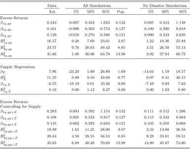
greater than zero and similar to the in-sample R2. Figure 1.3 shows the estimated slopes

windows for 2 year-ahead predictive regressions. We see that the estimates are stable, never

change signs, and are statistically significant in nearly all sub-samples. For comparison,

Figure 1.4 plots the same sub-sample betas for logP D. We see a lot of variation in the

estimated coefficients with numerous sign changes and weak statistical significance in

sub-samples (95% intervals straddle zero). The evidence suggests return predictability by GP

is robust both out-of-sample and over sub-samples. In Appendix A.1.1, I show that GP

is robust to finite-sample bias (Stambaugh (1999)) and size distortions (Torous, Valkanov,

and Yan (2004)). In Appendix A.1.2, I show that realized utility gains are high for

mean-variance investors using GP for portfolio allocation.

Gold and platinum are globally traded assets. This suggests that GP should also predict

future stock returns in international markets. I run the same predictive regressions as in

equation (1.1) using the MSCI World Index, which is a U.S. dollar denominated index

composed of stocks from 23 Developed Markets countries covering approximately 85% of

the free float-adjusted market capitalization in each country. Since the index is dollar

denominated, I use the U.S. Treasury bill rate as the risk-free rate. Table 1.7 shows that

the patterns of predictability are very similar to the U.S. results: high GP predicts high

future excess returns, although the coefficients are somewhat smaller in magnitude than for

U.S. returns. Since there may be some concern that the world portfolio consists of a large

proportion of U.S. stocks, I also run the same predictability regressions for other developed

countries. Panel B of Table 1.7 reports the results for the U.K., Switzerland, Japan, and

Sweden. I use the MSCI country indices for each of these countries, denominated in the

local currency. The risk-free rate is the local currency treasury bill rate. The results for

1.2.3. Dividend Growth Predictability

I have argued that stock return predictability by GP is driven by time variation in risk

premia and not from news about future dividend growth rates. Some may argue that

platinum has a characteristic not shared by gold: it is demanded by the automotive industry

for catalytic converters. Is it possible that it is actually bad news about the future cash

flows of car makers (GP is low when platinum is expensive, which is bad news for future

cash flows of car makers) that drives the predictability through a cash-flow channel? I run

standard dividend growth predictive regressions similar to Cochrane (2008) on real dividend

growth rates (∆dt) and real earnings growth rates (∆et):

12 h

h

X

i=1

∆dt+i=β0+β1logGPt+t+h

12 h

h

X

i=1

∆et+i=β0+β1logGPt+t+h

(1.4)

The results in Table 1.8 show no evidence of dividend growth predictability by GP.13 For

dividend growth, none of the estimated slopes from 1 year to 5 year horizons are statistically

different from 0, and the R2 are all nearly zero. For earnings growth, the R2 are slightly

higher but the t-statistics suggest the slopes are not significantly different from zero. This

is evidence that the predictability I document arises because of variation in risk premia

rather than dividend growth.

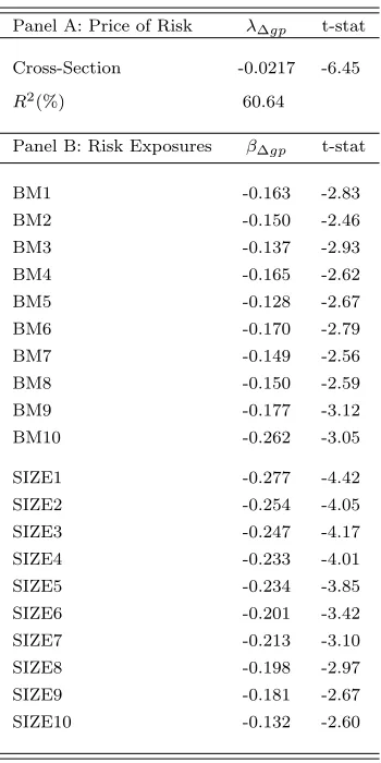
1.2.4. GP and the Cross-Section of Stock Returns

I examine the implications of GP risk for the cross-section of stock returns. As seen earlier,

GP is countercylical and increases in times of economic distress. Stocks with high, positive

covariation with GP innovations are therefore a good hedge against adverse states of high

economic risk and low asset valuations, which suggests that GP should command a negative

market price of risk in the cross-section. I estimate the risk exposures (betas) for each asset 13

i= 1, ..., N from time-series regressions

Re_i,t+1=ci+βi,∆gp∆ logGPt+1+i,t+1 (1.5)

whereRe_i,t+1 is the excess return for portfolio iand ∆ logGPt+1 = logGPt+1−Et[logGPt]

is the innovation in GP.14 _{The slope coefficient β}

i,∆gp represents the portfolio exposure of

asset ito GP risk. In order to estimate the cross-sectional market price of risk associated

with GP, I run a cross-sectional regression of time-series average excess returns on the risk

exposures

ERi,te +1

= cons +βi,∆gpλ∆gp+υi (1.6)

which yields estimates of the market price of risk λ∆gp. I use the standard cross-section of

ten portfolios sorted on the book-to-market ratio and ten portfolios sorted on size as my

test assets. The data is monthly from 1975 - 2013. Recall that GP is constructed without

any information from equity markets, which rules out any mechanical relationship between

GP risk and the cross-section of stock returns. Furthermore, the parsimonious one-factor

model avoids many statistical issues present in asset pricing tests that can mechanically

produce high explanatory power. Panel A of the Table 1.9 shows that the market price

of GP risk is significantly negative. Panel B of the Table further shows that the portfolio

returns are all significantly and negatively exposed to GP risk; equity returns decrease

contemporaneously when GP increases. The one-factor model featuring only GP risk can

explain over 60% of the cross-sectional variation in average returns. Figure 1.5 graphically

1.2.5. GP and Tail Risk

The evidence so far suggests that 1) GP is countercyclical and increases in times of

eco-nomic distress, 2) GP positively predicts future stock market excess returns, 3) GP risk is

negatively priced in the cross-section, and 4) GP is high when the default spread is high,

which is when firms with low credit ratings have higher probability of default. A plausible

interpretation consistent with these results is that GP captures tail risk in the economy.

This is broadly consistent with the findings of Manela and Moreira (2014), who use

ma-chine learning techniques to quantify tail risk (disaster concerns) from newspaper headlines:

“gold” is one of the top words which explains variation in investors’ tail risk concerns. GP

is persistent, which is consistent with the evidence of persistent tail risk in Kelly and Jiang

(2014). Options are an ideal way to measure tail risk because their convex payoff structure

contains rich information about the tail distribution of returns. I extract tail risk measures

from options markets and investigate the association between GP and tail risk.

Out-of-the-money (OTM) index put options protect against stock market crashes. The

slope of the implied volatility curve, defined as the implied volatility of an OTM put minus

the implied volatility of an at-the-money (ATM) put with the same maturity, is a measure

of tail risk in the economy (Pan (2002)). In the data, the implied volatility curve slopes

upward to the left since OTM puts are relatively more expensive (Rubinstein (1994)). I

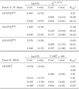
take the implied volatility curve from OptionMetrics and define SLOP E∆

t as the implied

volatility for an OTM put option between 20∆ to 40∆, which I subtract from the implied

volatility of an ATM put (50∆).15 The encompassing regression is:

SLOP E_t∆ | {z }

σ_t,IVOT M,∆−σAT M t,IV

=β0+β1logGPt+β2σAT Mt,IV +t.

(1.7)

To control for potential dependence of the slope on the level of implied volatility, I also

control forσAT M_t,IV on the right hand side of (1.7). Panel A of Table 1.10 shows the results.

15

We see that GP is significant for all definitions of the implied volatility slope, both by

itself and after controlling for the level of ATM implied volatility. The magnitude of the

coefficients as well as the t-statistics and R2 increase as the OTM put is further

out-of-the-money (more tail risk). An alternative measure of tail risk is the Bakshi et al. (2003)

model-free risk-neutral skewness. Bakshi and Kapadia (2003) and Jurek (2014) use this

measure as a proxy for crash risk; more negative skewness is associated with more crash

risk. The results in Panel B of Table 1.10 are similar to the results in Panel A: high GP

is associated with more negative risk-neutral skewness and GP is significant even after

controlling for the risk-neutral variance.

1.3. Gold and Platinum Markets

I examine key aspects of gold and platinum markets, including sources of demand for each

metal, the leasing markets, and return dynamics. Understanding the leasing markets is

important because no-arbitrage implies that investors are indifferent between buying gold

(platinum) or leasing gold (platinum) in perpetuity. Understanding the variation in rental

income will be important for the economic model and to compute gold and platinum returns.

1.3.1. Sources of Demand

Figure 1.6 shows the annual percentage demand for gold (top panel) and platinum (bottom

panel) for each of its major uses.16 From 1990 - 2013, approximately 70% of gold demand

was for jewellery, 15% for uses in technology (semiconductors, electronics), and 15% for

investments (coins, bars, ETF inventory building). Over the same period, approximately

40% of platinum demand was for jewellery, 15% for technology, while only a small fraction

the 1970s - securing sufficient supplies of platinum at stable prices became essential for

car makers. Black (2000) (Chapter 6) describes the long-term arrangements made between

platinum producers and car makers:

“With the introduction of autocatalysts...producers entered into long term

supply contracts with the auto manufacturers. Prices were negotiated on

con-tracts lasting up to five years”.

The private sale of platinum directly from producers to car makers means the amount of

platinum used in auto production does not enter the market. Therefore, net autocatalyst

demand (in excess of salvage) acts as negative platinum supply shocks since it reduces the

effective supply of platinum available for other uses. Under this view, the major source of

demand for gold and platinum comes from the jewellery industry.18

1.3.2. Lease Rates

Not surprisingly, jewellers are among the most active borrowers of gold and platinum. The

LBMA and LPPM describe the leasing market:

“The inventory loan is the basic financial tool of the precious metals

fab-ricating [industry]. For example, jewellery manufacturers can finance the raw

material in their production process by leasing gold...The same kind of strategy

would, for example, be adopted in platinum”.

Leasing is a convenient form of inventory financing widely practiced in both gold and

plat-inum fabrication industries (LBMA and LPPM (2008)). Le and Zhu (2013) find that over

the 1991 - 2007 sample, which purposely excludes the 2008 financial crisis to focus on normal

time dynamics, gold lease rates are increasing in stock market returns. This is consistent

with A¨ıt-Sahalia, Parker, and Yogo (2004) who document strong positive covariation

be-tween stock returns and demand for luxury goods. In normal times, gold lease rates are

combustion engines.

procyclical: as stock returns go up, jewellers have increased need for raw materials to meet

high demand for finished products and increase their gold borrowing, which drives up gold

lease rates.

The picture is different in times of economic distress. Figure 1.7 plots annualized gold

lease rates from 2007 - 2009. While gold lease rates are about 1% on average, the cost of

borrowing gold during the financial crisis jumped up threefold and high gold lease rates

persisted throughout the crisis. This is much greater than the observed decline in gold

prices during this period, which implies the rental income (economic value of holding gold)

must have been very high during the crisis. Several factors lead to countercyclical behavior

of lease rates in bad times. In severe economic conditions, lenders fear default by borrowers

and decrease the supply of loans, which increases the cost of leasing precious metals (LBMA

(2009)). Furthermore, to the extent that there are greater countercyclical benefits to service

flows from gold relative to platinum in bad times (for reasons discussed in the introduction),

expected gold rental income will exceed platinum. Risk premia are high in bad times, which

raises discount rates and lowers the prices of stocks, gold, and platinum. However, since gold

and platinum prices are equal to the discounted sum of future rental income, the increase

in expected gold rental income cushions the fall in gold prices relative to platinum prices.

1.3.3. Gold and Platinum Returns

Previous studies of gold returns (see e.g., Erb and Harvey (2013), Barro and Misra (2013))

focus only on the price appreciation of gold and do not include the rental income over the

ownership period. While Barro and Misra (2013) are correct in stating that gold dividends

and also the delivery options embedded in futures with physical settlement. I assume that

futures contracts will roll in the first week of the expiration month; it is estimated that only

1% to 2% of commodities futures contracts are actually delivered, so this approach should

not result in too much measurement error (Hirschey and Nofsinger (2008), Chapter 19). I

examine the resulting contract maturities and verify similar to Schwartz (1997) that the

maturities are relatively constant. The lease rate is given by:

Lease rate = Libor rate - Futures premium. (1.8)

Table 1.11 provides a table of cash flows analysis of the above from the perspective of a

jeweller, who is a typical borrower in the leasing market. For my analysis, I use futures

contracts closest to 3 months to maturity, and match it with the 3 month Libor rate to

calculate the lease rate, which I then annualize.20 I choose 3 month maturities to get a

contract with high liquidity, short time-to-maturity, yet not too short so that the physical

delivery option does not affect prices too much. I use average daily futures prices as the

monthly futures price, since my measure of monthly spot prices are average daily spot prices

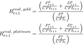
over the month. Real gold and platinum returns (inclusive of rental income) are calculated

in the standard way:

Rreal, gold_t+1 = _Pg

t+1

CP It+1 +

D_tg₊₁ CP It+1

_Pg t

CP It

Rreal, platinum_t+1 = _Px

t+1

CP It+1 +

Dtx+1

CP It+1

_Px t

CP It

(1.9)

where P_tg is the gold price, Px

t is the platinum price, D g

t is the gold rental income at time

t, andDx_t is the platinum rental income at timet, andCP Itis the consumer price index.21

The returns to gold and platinum can be interpreted from the perspective of an investor who

owns gold or platinum, and continuously leases the metal out, earning the rental income 20

Prior to 1986, I use Eurodollar deposit rates.

and any price appreciation. The results are summarized in Table 1.12. Average gold excess

returns are 2.40% per year, real gold return volatility is 16.76%, implying a Sharpe ratio of

0.14. Average platinum excess returns are 6.51% per year, real platinum return volatility is

22.18%, implying a Sharpe ratio of 0.29. For comparison, over the same period, the average

excess return for U.S. equities is 7.53% per year, real equity return volatility is 15.11%. The

gold risk premium is substantially lower than the equity risk premium. The risk premium

for platinum is slightly lower than equities as well, although the volatility is higher. Gold

lease rates are 1% per year on average. For comparison, Casassus and Collin-Dufresne

(2005) estimate the gold lease rate to be 0.9% per year, while Le and Zhu (2013) find an

average lease rate of about 1%. My estimate of the average platinum lease rate is 3.47%

per year. The economic model must match the low risk premium, high volatility, and low

lease rate of gold. At the same time, the model must also capture the relatively high risk

premium, high volatility, and high lease rate of platinum, while fitting the asset pricing

dynamics of equity markets and quantitatively accounting for the time variation and stock

return predictability of GP observed in the data.

1.4. Economic Model

1.4.1. Economic Environment

I analyze whether a general equilibrium model featuring time-varying disaster risk (Wachter

(2013)) and shocks to preferences for gold and platinum can jointly explain the empirical

facts documented in the previous sections. I assume an endowment economy with

com-plete markets and an infinitely-lived representative investor with Duffie and Epstein (1992)

I focus on the case of unit IES, which is done both for tractability, and consistent with

evidence in Vissing-Jørgensen (2002) and Hansen, Heaton, Lee, and Roussanov (2007).

Aggregate consumption growth is given by

dlogCt= ¯gcdt+σcdWtc+JtcdNtc (1.10)

where W_tc is a standard Brownian motion and N_tc is a Poisson process whose intensity λt

is given by a Cox, Ingersoll, and Ross (1985) square root process

dλt=κλ(ξt−λt)dt+σλ

p

λtdWtλ+JtλdNtλ (1.11)

where W_tλ a standard Brownian motion and N_tλ is a Poisson process whose intensity is

given by λλ

t =λt.23 Drechsler and Yaron (2011) use a similar framework to model jumps

in expected consumption growth and volatility. Allowing λt to jump allows stock prices

and volatility in the model to jump as well.24 This also allows the model to explain the

large observed jumps in volatility during the 2008 financial crisis as well as jumps in GP

seen in Figure 1.2.25 I solve for the stationary mean of λt in Appendix A.1.3. λt can be

approximately thought of as the probability of a consumption disaster.26 In the model,

market volatility is endogenously determined, and evidence from the volatility estimation

literature argues in favor of multiple time scales in volatility allowing for both long and

short run components.27 Also, as Seo and Wachter (2014) demonstrate, a one-factor model

without time-variation in the long-run mean of λt generates the counterfactual prediction

that the slope of the implied volatility curve decreases as the disaster intensity increases.

This arises because stock return volatility is endogenously determined and is driven by λt

23

Nowotny (2011) considers the implications of self-exciting intensity processes to model persistent disaster states. My setup differs since realized jumps in consumption do not trigger increases inλt.

24

This is consistent with the evidence in Duffie et al. (2000), Broadie et al. (2007), Eraker and Shaliastovich (2008), and Tauchen and Todorov (2011).

25

For parsimony, I do not distinguish explicitly betweenXt−andXtin my notation, as it should be clear from the context.

26_{The probability ofkjumps over an interval of time ∆t≈e}λt∆t(λt∆t)k

k! . 27

itself. To relieve this tension, and consistent with the evidence from the volatility estimation

literature, I follow Seo and Wachter and allow the long-run mean of λt to be a stochastic

processξt, which itself follows a square root process

dξt=κξ( ¯ξ−ξt)dt+σξ

p

ξtdWtξ (1.12)

whereW_tξ is a standard Brownian motion. All Brownian motions and Poisson processes are

assumed to be independent.

The size of the consumption jump,J_tcis drawn from the multinomial disaster distribution of

Barro and Ursua (2008), using data obtained from Robert Barro’s website. While the

mod-eling paradigm uses the rare disasters framework, the disasters I have in mind are smaller.

This will be made clearer in the following section when I discuss the model calibration.

The size of the jump in λt is given by Jtλ, which follows an exponential distribution with

meanµλ. Equity is modeled as a leveraged claim on aggregate consumption following Abel

(1999). The aggregate dividend at time t is Dt = Ctφ, for leverage parameter φ, which

implies that dividend growth dynamics are given by

dlogDt=φg¯cdt+φσcdWtc+φJtcdNtc. (1.13)

1.4.2. Gold and Platinum Supply

Gold and platinum do not depreciate, and consumption of the service flow from the stock

of gold and platinum today does not render it less capable of providing the same service

the aggregate per-capita gold and platinum stocks are smooth with no evidence of disasters,

and 2) the aggregate per-capita gold and platinum stocks are cointegrated.28 Given these

facts, I model logGt (the aggregate stock of gold) using a simple geometric Brownian

motion which is not subject to disasters. Consistent with the empirical evidence, logGt

and logXt(the aggregate stock of platinum) are modeled as cointegrated processes so that

logXt−logGt = logZt is a stationary process which itself follows an Ornstein-Uhlenbeck

process with long-run meanµz and reversion parameterθz:

dlogGt=µgdt+σgdWtg

dlogZt=θz(µz−logZt)dt+σzdWtz

logXt= logGt+ logZt.

(1.14)

All parameters for the gold and platinum supply dynamics are directly estimated from the

data.

1.4.3. Preferences

The representative investor’s utility function is defined recursively as

Vt=Et

Z ∞

t

f(Ωs, Vs)ds

forf(Ω, V) =δ(1−γ)V

log Ω− 1

1−γ log (1−γ)V

and Ωt=

C1−

1

t +αtG

1−1

t +βtX

1−1

t

1

1−1

(1.15)

wheref(Ω, V) describes the trade-off between current consumption Ωtand the continuation

utilityVt. The subjective time preference parameter isδ, andγ is commonly interpreted as

the coefficient of relative risk aversion.

The consumption aggregator Ωt is a constant elasticity of substitution (CES) aggregator

28

over nondurable consumption Ct, the gold stock Gt, and the platinum stock Xt.29 The

intratemporal elasticity of substitution is.30

The processes αt and βt capture in reduced-form time-varying preferences for gold and

platinum:

αt= exp(a1+a2λt)

βt= exp(b1+b2λt).

(1.16)

Specifically, αt and βt represent the relative importance of gold and platinum service flows

in the intratemporal consumption aggregator. Preference for precious metals responds to

changes in λt but not directly to ξt, since λt is the probability of a consumption disaster.

While the processesαtand βt gives me some additional flexibility, they depend completely

on existing state variables and no new state variables are being added. The parameter a2

(andb2) cannot be arbitrarily set. We want a relatively high value ofa2 to generate enough

countercyclical dynamics to match the low observed gold risk premium. However, when

a2 is too big, gold return volatility becomes too low, and gold lease rates will also be too

low. Additionally, existence of solutions for gold and platinum price-dividend ratios places

restrictions on the maximum a2 and b2 allowed, and this bound jointly depends on model

parameters such as the volatility and persistence of state variables, the severity of jumps,

and risk aversion. Changing these parameters to allow for higha2 will affect equity market

dynamics as well.31 29

The agent derives utility from gold and platinum service flows in direct proportion to its stock. This is a standard way to model preference for multiple types of goods, which has been used in the durable goods literature by Ogaki and Reinhart (1998) and Yogo (2006).

30_{I use a CES aggregator with the same elasticity of substitution across all pairs of goods for parsimony}

1.4.4. Asset Pricing

Duffie and Skiadas (1994) show that

πt= exp

Z ∞

0

fV(Ωs, Vs)d

fΩ(Ωt, Vt)

can serve as the state-price density in this economy. In equilibrium, the relationship between

Vtand the state variables is given by

Vt=

C_t1−γ 1−γe

a+bλλt+bξξt_.

In this economy, the equation for the state price density becomes

πt= exp(ηt−δbλ

Z t

0

λsds−δbξ

Z t

0

ξsds)δ Ω−tγea+bλλt+bξξt

where η = −δ(a+ 1) and a, bλ, bξ are the solutions to a system of equations given in

Appendix A.1.5. Following Barro and Misra (2013), I assume that outlays on gold and

platinum are negligible relative to nondurable consumption, which implies that Ωt ≈ Ct.

Under this assumption, the state price density is given by

πt≈exp(ηt−δbλ

Z t

0

λsds−δbξ

Z t

0

ξsds)δ Ct−γea+bλλt+bξξt (1.17)

The levels of αt and βt are small because per-capita expenditures on gold and platinum

are small compared to expenditures on nondurable goods and services. When the CES

aggregator is over multiple sources of consumption with large expenditure shares, such as

nondurable and durable consumption or housing, this approximation will become wildly

inaccurate; for example, Gomes, Kogan, and Yogo (2009) estimate the expenditure share

of durable goods to be 50%, in which case this assumption would not be innocuous. In

economic terms, the assumption implies that shocks to the supply of gold and platinum are

prices, but would conceivably not affect aggregate stock market risk premia, which seems

economically plausible. Going forward, I will assume that the approximation is accurate

and describe dynamics of the stochastic discount factor in (1.17) with an equality sign.

The instantaneous risk-free rate is given by

rf_t =δ+ ( ¯gc+

1 2σ

2

c)−γσc2+λtEv

h

e(1−γ)Jtc−_e−γJtc

i .

I follow Barro (2006) and Wachter (2013) and suppose that if a disaster occurs, the

gov-ernment will default on debt obligations with probability q, leading to a loss in the same

proportion as the consumption loss in the disaster.

The user costs (rental income) of gold and platinum are determined in equilibrium by the

intratemporal optimality conditions:

Qg,t=

ΩG

ΩC

= αt×

Ct

Gt

1

| {z }

countercyclical×procyclical

Qx,t=

ΩX

ΩC

= βt×

Ct

Xt

1

| {z }

countercyclical×procyclical

(1.18)

where Qg,t is the user cost of gold and Qx,t is the user cost of platinum. Notice from

equation (1.18) that the intratemporal elasticity of substitutionbehaves like the inverse of

the leverage parameterφ, since shocks to gold and platinum supply are small and unpriced.

When 1 < φ, gold and platinum will be safer than levered equity and command a lower

The same result holds in my model since gold and platinum supply shocks are unpriced.

This means that under the Barro and Misra (2013) assumption that > 1, the model

would predict that gold lease rates fall (gold prices rise) when the probability of a disaster

increases, which is counterfactual in light of Figures 1.1 and 1.7. Intuition suggests < 1

is more reasonable if we view gold and platinum as jewellery, since jewellery complements

nondurable consumption but does not substitute for it. Furthermore, >1 results in gold

return volatility being too low because in this case gold becomes a deleveraged consumption

claim. In my calibration, I set = _φ1 so that all the countercyclical properties of gold and

platinum arise through αt and βt.

Let Pt be the price of a claim to the stream of dividends Dt, and Ptt+τ be the price of the

asset which pays the single risky dividendDt+τ and nothing else. No arbitrage implies that

πtPtt+τ is a martingale, which implies that the equity price-dividend ratio is given by

Pt

Dt

= Z ∞

0

eaφ(τ)+bφ(τ)λt+cφ(τ)ξt_{dτ =G(λ}

t, ξt). (1.19)

Similar arguments hold for Pg,t and Px,t, which are the claims to gold and platinum,

re-spectively:

Pg,t

Qg,t

= Z ∞

0

eag(τ)+bg(τ)λt+cg(τ)ξt_{dτ =G}g_(λ

t, ξt)

Px,t

Qx,t

= Z ∞

0

eax(τ)+bx(τ)λt+cx(τ)ξt+dx(τ) logZt_{dτ =G}x_(λ

t, ξt,logZt).

(1.20)

The equity functions aφ(τ), bφ(τ), cφ(τ), gold functions ag(τ), bg(τ), cg(τ), and

plat-inum functionsax(τ), bx(τ), cx(τ), dx(τ) are given by the solution to systems of ordinary

1.4.5. GP in the Model

While I use the exact log GP ratio in my model simulations, a log-linearization conveys the

economic intuition more clearly.32

In Appendix A.1.6, I show that we can write log-linearized gold (Pg,t) and platinum (Px,t)

prices as

logPg,t=Ag+

1

logCt− 1

logGt+ (a2+b

∗

g,λ)

| {z }

<0

λt+ b∗g,ξ

|{z}

<0 ξt

logPx,t =Ax+

1

logCt− 1

logGt+ (b2+b

∗

x,λ)

| {z }

<0

λt+ b∗x,ξ

|{z}

<0

ξt+ (b∗x,Z −

1 ) | {z }

<0

logZt

(1.21)

where Ag, Ax, b∗g,λ, b∗g,ξ, b∗x,λ, b∗x,ξ, b∗x,Z are constants described in Appendix.1.6. Positive

shocks to logCtimply higher service flows and raise gold and platinum prices. The increase

is greater than the increase in consumption itself because of complementarity between

non-durable consumption and gold and platinum service flows (1 >1). High logGt lowers gold

prices since the quantity of gold becomes less scarce, and also lowers platinum prices due

to cointegration. Higher logZt means that (all else equal) the quantity of platinum is less

scarce, which also lowers platinum prices. Under my model calibration, strong discount rate

effects imply that, despitea2, b2>0, the overall response of gold and platinum to increases

inλtand ξt are negative, so that gold and platinum prices fall as disaster risks increase.

The log GP ratio is the difference between the log gold and platinum prices and is given by 32

The exact log GP ratio is given by

logGPt= log

Pg,t

Px,t

= log G

g (λt, ξt)

Gx_(λ

t, ξt,logZt)

Qg,t

logGPt= log

Pg,t

Px,t

= cons + (1 −b

∗

x,Z)

| {z }

>0

logZt+ (a2−b2+b∗g,λ−b∗x,λ)

| {z }

>0

λt+ (b∗g,ξ−b∗x,ξ)

| {z }

>0

ξt.

(1.22)

Shocks to logCt (which can be thought of as shocks to jewellery demand) affect gold and

platinum prices equally, leaving GP insulated from consumption shocks. Likewise, shocks

to logGt alone also cancel out and only the relative difference in supply logZt matters for

GP. Platinum is more expensive than gold on average because logXt <logGt on average

(platinum is more scarce). When logZt goes up, gold becomes scarce relative to platinum,

which increases GP. In the model, GP is increasing in both λt and ξt.33 High disaster

probabilities imply high risk premia, which leads to high discount rates and low equity

prices. Sincea2 andb2 are positive, the service flows from gold and platinum increase when

disaster probabilities increase, which partially offsets the higher discount rates and cushions

the fall in prices. This works similar to a cash flow effect, where the cash flow represents

gold and platinum rental income. Furthermore, a2 > b2 implies that the higher service

flow is greater for gold relative to platinum, which not only affects the immediate service

flow but also expected future service flow (rental income) through persistence in disaster

probabilities. This means that gold and platinum prices both fall as disaster probabilities

increase, but gold prices fall by less relative to platinum and GP is increasing in the disaster

probabilities. The fact that GP increases in λt and ξt allows the model to generate the

observed return predictability at both long and short horizons.

The logZt term is not priced by the stochastic discount factor but does affect the volatility

and persistence of GP. Stationarity of GP in the model is assured because logZtis stationary,

or in other words, because logGt and logXt are cointegrated. Interestingly, while shocks

to logZtaffect GP, they do not affect return predictability, which suggests that controlling

33

for logZt in the data can potentially lead to even stronger return predictability by GP. I

verify that this indeed holds in the data and discuss the results in the following section.

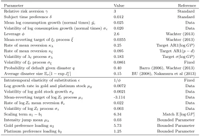
1.5. Calibration and Model Simulation Results

My parameter choices are given in Table 1.13. I have opted for smaller average jump sizes

with an average disaster size of 15%. Barro (2006) uses the dataset of Madison (2003) and

found the average disaster size to be 29%. Barro and Ursua (2008) update Madison (2003)

and find that the average disaster size is between 21-22%; this disaster distribution is also

used in Wachter (2013).34 I opt for smaller average disaster sizes in line with evidence

from Nakamura, Steinsson, Barro, and Ursua (2013), who document partial recoveries after

disasters, and estimate the average permanent impact of disasters to be about 15%. While

the actual probability of these smaller disasters is 5.85%, I opt for a more conservative

calibration of 4%, which is achieved using a ¯ξ = 0.0355 as in Wachter (2013) along with

an average jump size of µλ = 0.03 in the event of a jump in λt. Figure 1.8 compares my

multinomial jump size distribution with smaller average jump sizes to the distribution used

in Barro and Ursua (2008) and Wachter (2013). An important challenge in calibrating

representative investor models is to match the high observed volatility of the price-dividend

ratio. The model places an upper bound on the amount of volatility in the state variables

that can be allowed for solutions to exist (this is clearly seen in the equations for the

Epstein-Zin discount factor in Appendix A.1.5). I fix σξ such that the discriminant in the

solution to bξ is zero, which helps match the high volatility of the price-dividend ratio and

also reduces the number of free parameters. Theλtprocess is calibrated to be less persistent

volatility, low Sharpe ratio, and low lease rate. The model-implied gold lease rate is 0.93%,

which compares well to the 1% lease rate in the data. Lease rates in the model are the

convenience yield, which corresponds to the dividend yield (dividend over price). For

com-parison, I also present the model 90% confidence intervals for simulation paths in which

no disaster occurred. While these no-disaster intervals are more appropriate to compare

against stock and bond moments (since no disasters have occurred in the recent U.S. data,

on which the stock and bond returns are based), for gold and platinum returns it is more

natural to compare against population moments, since there have been 21 economic

dis-asters from 1975 - 2006 in international markets (using my disaster cutoff) based on the

Barro and Ursua (2008) dataset (including several OECD countries), which can

conceiv-ably affect gold and platinum returns and volatilities. The model explains the expected

returns, volatilities and lease rates for platinum as well, including the high lease rate and

high volatility. The model also accounts for time variation in GP, with the volatility and

persistence of GP falling right inside the 90% confidence intervals. The median persistence

for all simulations matches the data estimate nearly perfectly. Following this, I run the

below return predictability regressions using model excess stock returns and GP:

1 h

h

X

i=1

log(R_te_+i)−log(Rb_t+i) =β0+β1log(GPt) +t+h.

The left hand side is the normalized excess return for one year up through five years ahead,

while the right hand side is the model GP. The results are shown in the top panel of

Table 1.15. The data estimates fall right in the model confidence intervals, with the data

R2 estimates very close to the median values.35 Thus, the model can explain the observed

predictability of returns by GP. Similar to the data, the model delivers very low to negligible

dividend growth predictability, similar to (Wachter (2013)). The model can also account

for the observed relationship between GP and the slope of the implied volatility curve for

index options, as detailed in Appendix A.1.7.

35_{It is difficult to decide which, all simulations or no disasters, is most appropriate for the predictability}

How well have I captured the effect of supply dynamics on GP? Is there predictability coming

from the supply effects (including autocatalyst demand)? The second panel of Table 1.15

investigates this issue. I regress GP on logZt inside the model, and we see that the data

estimate falls right inside the 90% interval.36 Since the leading coefficient on logZt in the

model depends on 1, this serves as a further check on the assumed complementarity ( <1)

between jewellery (gold and platinum) and nondurable consumption. Under a calibration

where >1 as in Barro and Misra (2013), this regression in the data results in a coefficient

smaller than 1. The second regression in this panel investigates return predictability by

logZt in both the model and the data. In the model, logZt does not predict returns by

construction, although in small samples it is occasionally possible to spuriously find weak

evidence of predictability. Both the population and median values, however, show that

there is no predictability coming from the supply channels. I run the same regression in the

data and find no evidence of predictability through logZt, which is further evidence that

the predictability does not come from a cash flow channel.

These results for repeated samples of 39 years lead to an interesting finding. Time-variation

in GP over finite samples is affected by logZt, which is not a priced variable in this economy.

The third panel shows return predictability regressions where I control for the effect of logZt,

which adds volatility and persistence to GP without adding predictive power. We see in

this case that the point estimates increase at all horizons, and now the 90% interval for

return predictability by GP does not contain 0. The R2 increase over all horizons quite

dramatically. In the data, we can separately identify logZt and logAt, the aggregate

per-capita stock of platinum used as autocatalysts. Empirically, a regression of GP on logZt