Design of Intrusion Detection System Based on Improved
ABC elite and BP Neural Networks
Letian Duan, Dezhi Han, and Qiuting Tian
College of Information Engineering, Shanghai Maritime University Shanghai 201306, China
[email protected], [email protected], [email protected]
Abstract. Intrusion detection is a hot topic in network security. This paper pro-poses an intrusion detection method based on improved artificial bee colony al-gorithm with elite-guided search equations (IABC elite) and Backprogation (BP) neural networks. The IABC elite algorithm is based on the depth first search frame-work and the elite-guided search equations, which enhance the exploitation ability of artificial bee colony algorithm and accelerate the convergence. The IABC elite algorithm is used to optimize the initial weight and threshold value of the BP neu-ral networks, avoiding the BP neuneu-ral networks falling into a local optimum during the training process and improving the training speed. In this paper, the BP neural networks optimized by IABC elite algorithm is applied to intrusion detection. The simulation on the NSL-KDD dataset shows that the intrusion detection system based on the IABC elite algorithm and the BP neural networks has good classification and high intrusion detection ability.
Keywords:Intrusion Detection, Machine Learning, BP Neural Networks, Improved ABC elite.
1.
Introduction
With the development of network technology, especially the widespread use of the In-ternet, it is more convenient to interconnect and interoperate. However, the problem of network security is also becoming increasingly prominent, and lawbreakers may seek benefits through damage to the network. Therefore, the detection and defense of network attacks is a hot topic of network security. Attackers usually leverage network protocol vul-nerability to perform network attacks, including Denial of Service (DoS), User to Root (U2R), Probe and Root to Local (R2L). So far, methods for detecting network attacks include classification and clustering, which detect network attacks by analyzing network data flow.
has been widely used in prediction, modeling, classification, adaptive control and other fields.
The Swarm intelligence is simply defined as the collective behavior of decentralized and self-organizing swarms. As we all know, these swarms can be birds, fish and the colony of social insects such as ants and bees. In the 1990s, especially two methods, based on the ant colony and bee colony, attracted the interest of researchers. The Swarm intelligence requires a colony to meet self-organizing features. Since the 21st century, re-searchers have started to be interested in new intelligent methods using bee colony behav-ior. In the past decade, some algorithms based on various intelligent behaviors of honey bee colony have been proposed. The population algorithm originates from the resolution of numerical optimization problems and is a meta-heuristic target optimization algorithm. In view of the shortcomings of traditional neural network training methods, researchers began to try to apply heuristic search algorithms to artificial neural network design and parameter optimization. That is to say, heuristic search methods can be used to train neu-ral networks. The fusion of the heuristic search algorithms and neuneu-ral networks are called evolutionary neural networks [29,30]. Artificial Bee Colony Algorithm (ABC) is a new heuristic search algorithm. It was proposed at Erciyes University in 2005. The algorithm is derived from the research and simulation of honey bee collective behavior. Compared with other heuristic search algorithms such as Particle Swarm Optimization (PSO), Ant Colony Optimization (ACO) and Differential Evolution (DE), ABC algorithm is simple, robust as well as need few parameters.
The optimization technology is an application technology that uses mathematics as the basis to find the optimal feasible solution for the objective optimization problem un-der certain conditional constraints. Before the 1980s, the optimization algorithms mainly were used to mathematical analysis, iterative solution and other methods to solve practi-cal problems. They were practi-called traditional optimization algorithms. These methods have complete theoretical analysis and mathematical proofs, and have also achieved good re-sults in optimization problems such as continuous and low-dimension. But they seem to be powerless for multi-peak, high-dimension and discontinuous optimization problems. From the 1980s, some novel heuristic search algorithms emerge, which are different from traditional optimization algorithms. For example, the Genetic Algorithm is a computa-tional model that simulates the natural selection and genetic mechanism of Darwin bi-ological evolution. The idea of Simulated Annealing algorithm comes from the process of solid material annealing in physics. All these algorithms simulate some processes that occur in nature.
experiment results. We analyze the experiment results in detail. Finally, the conclusion is discussed in Section 7.
2.
Related Work
The artificial bee colony algorithm is a heuristic swarm intelligence algorithm designed by Karaboga in 2005 to mimic the collective behavior of the honey bee. It was originally designed to solve some numerical optimization problems [12]. The artificial bee colony algorithm was used to optimize multivariate functions, and compared with algorithms such as genetic algorithm (GA) and particle swarm optimization (PSO). The results show that ABC is superior to other algorithms [14]. However, the artificial bee colony algorithm is good at exploring the solution, but it is poor in exploitation and easy to fall into a local optimum. Ref. [32] proposed an improved ABC algorithm called gbest-guided artificial bee colony (GABC) algorithm, which combines the information of the global optimal so-lution into the soso-lution search equation to improve the exploitation. Ref. [27] proposed a multi-strategy ensemble artificial bee colony (MEABC) algorithm. In MEABC, a pool of distinct solution search strategies coexist throughout the search process and compete to produce offspring. The MEABC method effectively improves the performance of ABC on continuous optimization problems. Ref. [2] proposed an artificial bee colony algo-rithm with Elite-Guided Search Equations combined with a depth-first framework, named DFSABC elite. Prioritizing more computing resources for better solutions enhances the exploitation capabilities of the algorithm.
The use of artificial bee colony algorithm to train artificial neural networks also has a certain historical background. In Ref. [13], the artificial bee colony algorithm is used to train neural networks to solve the benchmark problems of XOR, 3-bit parity, 4-bit encoder-decoder, etc., which embodies the ability of artificial bee colony algorithm to train neural networks. Ref. [21] proposed a hybrid algorithm combining artificial bee colony algorithm and Levenberq-Marquardt algorithm (ABC-LM) to train artificial neu-ral networks. The neuneu-ral network is first trained with ABC, and then LM continues to train the neural network using the optimal weight set of the ABC algorithm and attempts to minimize training errors. The results of the experiments show that the hybrid ABC-LM algorithm has better performance. However, this method has only been tested on bench-mark issues such as XOR, 3-bit parity, 4-bit encoder-decoder, etc., and has not been tested on high dimensional classification benchmark problems.
In 1999, Wenke et al. applied the machine learning method to intrusion detection for the first time. By analyzing the network data traffic, an anomaly detection model was ob-tained [18]. In Ref. [23], a distributed denial of service attack (DDos) detection method based on BP neural network is proposed, which is carried out by simple traffic classi-fication and feature selection. The detection of DDos traffic reaches a certain detection rate. However, this method has a long training time and is easy to falling into a local op-timum. Ref. [31] proposed a recurrent neural network (RNN) deep learning method for intrusion detection, which was simulated in binary-classification and multi-classification environments, but the method still needs to improve the detection accuracy and reduce the training time of the neural network model.
DFSABC elite algorithm by integrating the Gaussian search equation in Ref. [19] into the DFSABC elite algorithm, which improves the exploitation ability of the artificial bee colony algorithm and accelerates the search for the optimal solution. The use of IABC elite to optimize the BP neural network avoids the neural network falling into lo-cal optimum and solves the problem of slow convergence of neural network training to some extent. The intrusion detection method based on IABC elite and BP neural network improves the accuracy of intrusion detection and reduces the false positive rate. In the NSL-KDD dataset, KDDTrain+ and KDDTest-21 were respectively selected as training dataset and testing dataset to verify the performance of the algorithm.
3.
BP Neural Networks
The Artificial Neural Network is an intelligent algorithm by simulating the structure of the neural system and information delivery of biological neural networks. Each single neuron performs simple operations. When numerous neurons are combined and operated together, they make up a huge distributed and parallel computing model.
3.1. Neuron Model
Neurons are basic information processing units for neural networks. Fig. 1 shows a model of a neuron which is the basic unit of artificial neural networks. The neuron model com-prises three basic elements:
1) Synapses, each of them are characterized by its weight value. In particular, the synaptic weight valuewij is a coefficient that multiplies the input signal xi. The first subscript of the weight value refers to the query neuron, and the second subscript refers to the receptor neuron where the weight value is located.
2) A linear combiner, it is for summing the input signals multiplied by the weight value of the corresponding synapse according to Eq.(1).
netj = m
X
i=1
wijxi+θj (1)
Wherexiis theith component of the input signal,mis the dimension of the input sig-nal,wij is theith component of the synaptic weight value of neuronj,θjis the threshold value of neuronj, andnetjis the output value of the linear combiner.
3) The activation function, which limits the amplitude of the neuron output signal and limits the value to a certain value within the allowable range. In general, the normal amplitude of a neuron output signal value is in the range of [0, 1] or [-1, 1].
The output signal valueyjof the neuron model is calculated according to Eq.(2).
yj=ϕ(netj) (2)
3.2. Multilayer Feedforward Neural Networks
... 1 x
2 x
m
x
...
Activation function
Output Threshold value
Input signal
Synaptic weight value 1j
w
2j
w
mj
w
j
y
j
( )
Fig. 1.Neuron model
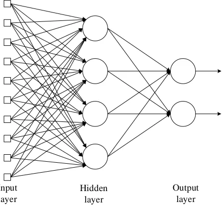
the neuron of the output layer, rather than the opposite, which is called the feedforward neural networks. A multilayer feedforward neural network refers to one or more layers of hidden neurons in the neural network.
Input layer
Hidden layer
Output layer
Fig. 2.Three-layer feedforward neural networks
nodes, 4 hidden neurons, and 2 output neurons. In general, a feedforward neural network has msource nodes, hneurons in the hidden layer andqneurons in the output layer, which can be calledm-h-qneural networks. The output signal of output layerkth neuron is calculated according to Eq.(3).
zk=ϕ2
h
X
j=1
wjkϕ1
m
X
i=1
wijxi+θj
!
+θk
(3)
Whereϕ1(·)is the activation function of the hidden layer neuron, andϕ2(·)is the
activation function of the output layer neuron.
3.3. Backpropagation Algorithm
Backpropagation (BP) algorithm is a common method to train artificial neural networks based on the gradient descent method. The gradient descent method minimizes the loss function by updating weight values and threshold values toward the fastest direction. Here, we derive the increment of weight values and threshold values.
For convenience of description, we use the square error function as the loss function according to the Eq.(4).
J(w) = 1 2
q
X
k=1
(tk−zk)
2
= 1
2||t−z||
2 (4)
Wheret andzare the target vector and the neural networks output vector whose length isq,wrepresents all the weight values in the neural networks.
The backpropagation rule is based on the gradient descent method. In the beginning, the weight values are initialized to random values and then adjusted toward the direction of reducing the error value.
∆w=−η∂J
∂w (5)
This can be expressed in the form of a component,
∆wpq=−η ∂J ∂wpq
(6)
Whereη is the learning rate, which represents the relative change ratio of the weight values. We consider Eq.(6) in the three-layer neural networks.
1) We use the chain differentiation rule to entail the update rules of weight values and threshold values from the hidden layer to the output layer.
∂J ∂wjk
= ∂J
∂netk ∂netk
∂wjk
=−δk ∂netk
∂wjk
(7)
The sensitivity degree of unitkis defined as
δk =− ∂J ∂netk
This sensitivity degree describes that the total error varies with the activation of the unit.
δk=− ∂J ∂netk
=−∂J
∂zk ∂zk ∂netk
= (tk−zk)ϕ20(netk) (9)
And due to
∂netk ∂wjk
=yj (10)
So
∆wjk=ηδkyj=η(tk−zk)ϕ20(netk)yj (11)
Same reason
∆θk =η(tk−zk)ϕ20(netk) (12)
2) We entail the update rules of weight values and the threshold values from the input layer to the hidden layer.
∂J ∂wij
= ∂J
∂yj ∂yj ∂netj
∂netj ∂wij
(13)
Where
∂J ∂yj =
∂ ∂yj
1 2
q
P
k=1
(tk−zk)
2
=−
q
P
k=1
(tk−zk)∂z∂ykj
=−
q
P
k=1
(tk−zk)∂net∂zkk∂net∂yjk
=−
q
P
k=1
(tk−zk)ϕ20(netk)wjk
(14)
So
∆wij =η
" q
X
k=1
wjkδk
#
ϕ10(netj)xi (15)
Same reason
∆θj =η
" q
X
k=1
wjkδk
#
ϕ10(netj) (16)
4.
Artificial Bee Colony Algorithm
The artificial bee colony algorithm (ABC) is an algorithm that simulates honey bee collec-tive behavior. Its role is divided into employed bee, onlooker bee, and scout bee. Assume that in theDdimensional space, the population size is2×SN ,SN is the number of honey sources (employed bee number = onlooker bee number =SN). The honey sources and the employed bees correspond one to one, that is to say, the number of honey sources isSN, and the position of theithsource of honey is denoted asxi. Each honey source location represents a candidate solution to the optimization problem, and the fitness of the honey source reflects the quality of the solution.
4.1. Four Phases of Artificial Bee Colony Algorithm
Initialization phase: At the beginning of the ABC, the initial food sources are generated
randomly according to Eq.(17).
Xi,j=XjL+randj(XjU−X L
j) (17)
Wherei={1,2, . . . , SN},j ={1,2, . . . , D},XjLandXjU are the upper and lower bounds of thejthvariable respectively.randj is a random value in the range of [0,1]. Then, the fitness value of the food sources are calculated by Eq.(18).
f iti=
1
1+f(Xi) f(Xi)≥0
1 +|f(Xi)|f(Xi)<0
(18)
Wheref itiis the fitness value of the food sourceXi,f(Xi)is the objective function value of food sourceXifor the optimization problem. In addition, parameterlimitshould be determined. The parameter counter records the number of unsuccessful updates, is initialized to 0 for each food source.
Employed bee phase: Each Employed bee will fly to a distinct food source, looking
for a candidate food source around the corresponding food source by using Eq.(19).
Vi,j=Xi,j+φi,j×(Xi,j−Xk,j) (19)
Whereiandkare randomly selected from{1,2, . . . , SN},j is randomly selected from{1,2, . . . , D},Vi,j is thejthdimension of theithcandidate food source;Xk,j is thejthdimension of thekthfood source,φi,jis a random real number in the range of [-1,1].
After finding a new food source, the fitness value of the candidate food source is calculated by Eq.(18). If the candidate food source has a fitness value superior to the old food source, the food source replaces the old food source and the corresponding employed bee memorizes a new food source, and thecountervariable of this food source is reset to 0. Otherwisecounteris increased by 1.
Onlooker bee phase: According to the quality information of the food source shared
pi= f iti
PSN i=1f iti
(20)
Obviously, the value of fitness is greater, the selection probability is higher. If a can-didate food sourceVsobtained by the onlooker bee is superior to the food sourceXs,Xs will be replaced by the new food source. And thecountervariable of the food source is reset to 0. Otherwisecounterof the food source is increased by 1.
Scout bee phase: A food source with a highestcountervalue is selected and compared
with a predefinedlimitvalue. If the value is greater than the value oflimit, the selected food source is abandoned by its employed bee, and the employed bee is converted to a scout bee, and then this scout bee randomly finds a new source of food according to Eq.(17). After acquiring a new food source, the correspondingcounteris reset to 0 and the scout bee is changed to employed bee. Note that if thejthvariableVi,j of theith candidate food source violates the upper and lower bound constraints in the employed bee phase and the onlooker bee phase, the food source is reset according to Eq.(17).
4.2. The Improved ABC elite Algorithm
ABC algorithm is a population-based, iteration-based and stochastic optimization algo-rithm, and it is very effective for solving numerical optimization problems. However, al-though the search equations are stronger in exploration, insufficient in exploitation. And the convergence performance of the ABC algorithm is not prominent. So, in order to bet-ter balance exploration and exploitation, Ref. [2] proposed a Depth First Search (DFS) framework and two search equations based on elite solutions, as shown in Eq.(21) and Eq.(22). This method named DFSABC elite. The DFS framework can prioritize more computing resources to better solutions to enhance the exploitation ability of the algo-rithm. The elite-guided search equations keep the solution with the highest fitness value in the iteration, which speeds up the training process of the algorithm.
Vi,j=Xe,j+φi,j×(Xe,j−Xk,j) (21)
Ve,j =
1
2(Xe,j+Xbest,j) +φe,j×(Xbest,j−Xk,j) (22)
WhereXeis a randomly selected solution from the elite solution, andXk is a ran-domly selected solution from the current population.eis not equal tok, andkis not equal toi.Xbestis the current best solution.φi,j,φe,jare two random real numbers in the range of [-1, 1].
In order to better balance ABC exploration and exploitation capabilities, Ref. [6] ad-dresses the problem that the candidate solution search equation has too large a disturbance to the elite solution in the search equation proposed in Ref. [2], and proposes an elite search equation. The candidate solutions for solutions and ordinary solutions should use different search equations. Ref. [17] proposed a novel search equation in Particle Swarm Optimization (PSO) algorithm, as shown in Eq.(23).
Pi=
c1×pbesti+c2×gbest
c1+c2
Wherec1andc2are two learning coefficients,pbestis the personal best position, and
gbestis the population best solution found so far. Based on Eq.(23), a novel equation is proposed in Ref.[19].
Xi=N
gbest+pbest
i
2 ,|gbest−pbesti|
(24)
WhereN represents the Gaussian distribution, gbest+pbesti
2 represents the mean, and |gbest −pbesti| represents the standard deviation. The information around pbest and gbestis exploited by using the Gaussian distribution in Eq.(24). A similar Gaussian search equation is proposed according to Eq.(24).
Vi,j=N
X
best,j+Xi,j
2 ,|Xbest,j−Xi,j|
(25)
WhereXi,jis thejthelement of the elite solutionXi;Xbest,jis thejthelement of the global best solution found so far, andjis randomly selected from{1,2, ..., D}. According to Eq.(25), the elite solutions in employed bee phase search aroundXbestcan improve the exploitation ability of ABC and the success rate of disturbance for elite solutions.
The search equation for the elite candidate solution is shown in Eq.(26).
Ve,j=
1
2(Xe,j+Xbest,j) +φe,j(Xbest,j−Xe0,j) (26)
The elite-guided search equations enhance ABC algorithm ability for exploiting solu-tions. The DFSABC elite algorithm is combined with the two novel elite-guided search equations forming a new ABC variant called the Improved ABC elite Algorithm (IABC -elite).
Algorithm 1The procedure of IABC elite
1: Initialization: GenerateSNsolutions that contain variables according to Eq.(17); 2:whileF es <max F esdo
3: Select the top solutions as elite solutions from populations; 4: fori= 1toSNdo
5: //employed bee phase 6: ifiis an elite solutionthen
7: Generate a new candidate solutionViin the neighborhood ofXi using Eq.(24);
8: else
9: Generate a new candidate solutionViin the neighborhood ofXi using Eq.(21);
10: end if
11: Evaluate the new solutionVi; 12: iff(Vi)< f(Xi)then 13: ReplaceXibyVi; 14: counter(i)=0; 15: else
16: counter(i)=counter(i)+1;
17: end if
18: end for//end employed bee phase
19: fori= 1toSNdo
20: //onlooker bee phase
21: Select a solutionXefrom elite solutions randomly to search; 22: P0= 1−F es/max F es
23: ifrand(0,1)< P0then
24: Generate a new candidate solutionVein neighborhood ofXein neighborhood ofXeusing Eq.(22)
25: else
26: Select a solutionXe0 from elite solutions randomly, wheree0not
equal toe;
27: Generate a new candidate solutionVeusing Eq.(26);
28: end if
29: Evaluate the new solutionVe; 30: iff(Ve)< f(Xe)then 31: ReplaceXebyVe; 32: counter(e)=0; 33: else
34: counter(e)=counter(e)+1;
35: end if
36: end for//end onlooker bee phase
37: F es=F es+SN∗2
38: Select the solutionXmaxwith max counter value; //Scout bee phase
39: ifcounter(max)> limitthen
40: ReplaceXmaxby a new solution generated according to Eq.(17);
41: F es=F es+ 1,counter(max) = 0
5.
BP Neural Networks Based on IABC elite Algorithm
The Backprogation (BP) neural network based on IABC elite algorithm is the combina-tion of improved bee colony algorithm and BP neural networks algorithm. A new BP neural network optimized by improved ABC elite algorithm is proposed and applied to intrusion detection. The research results of numerous papers show that the BP neural networks are sensitive to initial parameters [25,29,30]. Although there are many papers use particle swarm optimization (PSO), genetic algorithm (GA) and other algorithms to optimize the initial parameters of BP neural networks, the IABC elite algorithm better balance the exploration and exploitation ability of the solution. With the strong ability to jump out of the local optimal solution, so using IABC elite to optimize BP neural network can further improve the performance of BP neural networks. The optimized objection for IABC elite algorithm are the weight values and threshold values of the neural networks. This method can improve the self-learning ability of BP neural network and speed up the convergence process of Backpropagation algorithm, so the neural network intrusion detection model have better detection ability. Its key techniques lie in:
Use the IABC elite algorithm to train the neural network to generate the initial weight values and threshold values of the neural networks and use the error function of the neural networks as the fitness objective function of the IABC elite algorithm.
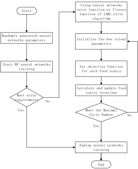
The food source position in the IABC elite algorithm represents the weight values and threshold values in the BP neural networks. The fitness value of each food source is calcu-lated through the fitness function, which is the error function of the neural networks. The food source has a lower error value, has a higher fitness value. The IABC elite algorithm tends to select the higher fitness value food source. The IABC elite algorithm finds the honey source of the best fitness value in the search process. The best honey sources are obtained by comparing the current fitness value and historical value of each honey source within the process of iterations. The best honey source will be set as the initial weight val-ues and threshold valval-ues of the BP neural network. When the error function value of the neural network generated by the best honey source meets the error precision requirement, the backpropagation algorithm performs further training for the neural network and tries to minimize the training error value. The algorithm avoids the neural network falling into a local optimum, achieves the goal of improving the accuracy and speeds up the neural network training. The basic idea of using IABC elite algorithm to optimize BP neural network as follows:
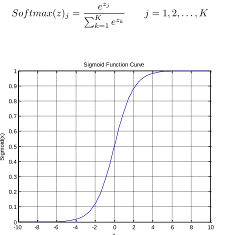
First, we construct a neural network model, set the number of nodes in the input layer and the number of neurons in the hidden layer and the output layer. And construct the connection between the input layer and the hidden layer, as well as the hidden layer and the output layer. The activation function of the hidden layer neuron is set as Sigmoid function. The function equation is shown in Eq.(27), and the Sigmoid function curve is shown in Fig. 3. The Sigmoid function curve is S, which can map the output signal value of the linear combiner to the range of [0, 1].
Sigmoid(x) = 1
1 +e−x (27)
Sof tmax(z)j= ezj
PK
k=1ezk
j= 1,2, . . . , K (28)
-10 -8 -6 -4 -2 0 2 4 6 8 10 0
0.1 0.2 0.3 0.4 0.5 0.6 0.7 0.8 0.9 1
x
S
ig
m
o
id
(x
)
Sigmoid Function Curve
Fig. 3.Sigmoid Function Curve
Second, the IABC elite algorithm is used to train the neural network and generate initial weight values and threshold values for the neural network. Set the population size of the IABC elite algorithm and set the dimension of the solution according to the number of variables in the threshold values and weight values of the neural network. The position of the food source represents the weight values and threshold values of the neural network. The neural network error function is used as the food source fitness value function. High fitness food sources are those food sources with high fitness weight values and threshold values. The IABC elite algorithm obtains a better solution by updating the honey sources during the iterative process. Table 1 show the mapping relation between neural networks training parameter and honey bee collective behavior. The IABC elite algorithm choose the best fitness food source as the initial weight values and threshold values of the neural network.
Table 1.Mapping relation between neural networks training parameter and honey bee collective behavior
honey bee collective behavior neural networks training parameter
Finally, the backpropagation algorithm trains the neural network according to the ini-tial weight values and threshold values generated by IABC elite algorithm. The backprop-agation algorithm tries to minimize the training error by gradient descent. The weights and thresholds with the smallest training error will be used as parameters of the neural network for intrusion detection of network traffic.
The detail algorithm process is described as follows:
1) Select sample data for training, and randomly generate the weight valueswij be-tween the input layer neurons and the hidden layer neuron, the weight valueswjkbetween the hidden layer neurons and the output layer neurons. As well as generate the threshold values θj of the hidden layer neurons and the threshold values θk of the output layer neurons.
2) The output values of neural networks output layer neurons are calculated according to Eq.(29), Eq.(30), Eq.(31), and Eq.(32).
netj = m
X
i=1
wijxi+θj (29)
yj=ϕ1(netj) (30)
netk= h
X
j=1
wjkyj+θk (31)
zk =ϕ2(netk) (32)
3) The error of the neural network is calculated according to Eq.(33). If it meets the required error, end training and go to step 5); otherwise go to step 4).
J(w) = 1 2
q
X
k=1
(tk−zk)2 (33)
4) The weight values and threshold values between the hidden layer and the output layer are adjusted according to Eq.(34) and Eq.(35). The weight values and threshold values between the input layer and the hidden layer are adjusted according to Eq.(36) and Eq.(37).
∆wjk=η(tk−zk)ϕ20(netk)yj (34)
∆θk =η(tk−zk)ϕ20(netk) (35)
∆wij =η
" q
X
k=1
wjkδk
#
ϕ10(netj)xi (36)
∆θj =η
" q
X
k=1
wjkδk
#
ϕ10(netj) (37)
δk=− ∂J ∂netk
=−∂J
∂zk ∂zk ∂netk
= (tk−zk)ϕ20(netk) (38)
5) From the results obtained in step 4), we can get the new weight valueswij and the new threshold valuesθj between the input layer and the hidden layer, as well as the new weight valueswjkand the new threshold valuesθkbetween the hidden layer and the output layer.
Start
Randomly generated neural networks parameters
Meet error requirements Start BP neural networks
training
Using neural networks error function as fitness
function of IABC_elite algorithm
Initialize the bee colony parameters
Set objective function for each food source
Calculate and update food source locations
Meet the Maximal Cycle Number
Ending neural networks training
End Yes
No
Yes
No
Fig. 4.Flowchart of IABC elite algorithm to optimize BP neural networks
6) According to the new weight values and threshold values, re-execute step 1) to 3). If the error meets the requirements, end the training process. Otherwise, continue.
7) Using the current weights and thresholds as neural work input signal, and get the corresponding neural network output signal. The neural network loss function is set as the objective function of Eq. (39). Set the value of the Max Cycle Number (M CN).
f iti=
1
1+f(Xi) f(Xi)≥0
1 +|f(Xi)|f(Xi)<0
8) Run the IABC elite algorithm until iterations reaches the maximum number of iter-ationsM CN. Set the weight values and threshold values from the IABC elite algorithm as new initial parameters to train the neural network, then go to step 4).
9) End the training process; output the weight valueswij and the threshold valuesθj as well as the weight valueswjk and the threshold valuesθk. Use the obtained neural networks model for testing data to predict the classification.
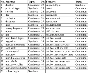
Table 2.Features of NSL-KDD datasets
No. Features Types No. Features Types
1 duration Continuous 22 is guest login Symbolic
2 protocol type Symbolic 23 count Continuous
3 service Symbolic 24 srv count Continuous
4 flag Symbolic 25 serror rate Continuous
5 src bytes Continuous 26 srv serror rate Continuous 6 dst types Continuous 27 rerror rate Continuous 7 land Symbolic 28 srv rerror rate Continuous 8 wrong fragment Continuous 29 same srv rate Continuous 9 urgent Continuous 30 diff srv rate Continuous 10 hot Continuous 31 srv diff host rate Continuous 11 num failed logins Continuous 32 dst host count Continuous 12 logged in Symbolic 33 dst host srv count Continuous 13 num compromised Continuous 34 dst host same srv rate Continuous 14 root shell Continuous 35 dst host diff srv rate Continuous 15 su attempted Continuous 36 dst host same src port rate Continuous 16 num root Continuous 37 dst host srv diff host rate Continuous 17 num file creations Continuous 38 dst host serror rate Continuous 18 num shells Continuous 39 dst host srv serror rate Continuous 19 num access files Continuous 40 dst host rerror rate Continuous 20 num outbound cmds Continuous 41 dst host srv rerror rate Continuous 21 is host login Symbolic
6.
Experiments and Analysis
6.1. Dataset Description
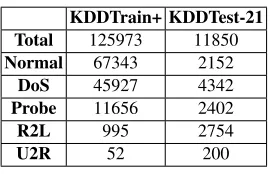
and abnormal network data ratios makes the testing and training data more reasonable, making it more suitable for efficient evaluation of different machine learning techniques. Table 2 shows the features of the NSL-KDD dataset. NSL-KDD dataset contains train-ing dataset KDDTrain+.txt, KDDTrain+ 20Percent.txt. KDDTrain+ 20Percent is 20% of KDDTrain+ data. NSL-KDD dataset contains testing dataset KDDTest+.txt, KDDTest-21.txt. The test accuracy is generally less than KDDTest+ on KDDTest-21. The number of samples of different classifications of the NSL-KDD dataset shows in Table 3.
Table 3.Different Classifications of NSL-KDD Dataset
KDDTrain+ KDDTest-21
Total 125973 11850
Normal 67343 2152
DoS 45927 4342
Probe 11656 2402
R2L 995 2754
U2R 52 200
6.2. Data Preprocessing
1) Vectorization
The NSL-KDD dataset has 34 numeric features and 7 symbol features. The features of 2, 3, 4, 7, 12, 21, and 22 columns are the symbol features, where the features of 7, 12, 21, and 22 columns are ‘0’ or ‘1’, and the features of 2, 3, and 4 columns are the character type. Because the input value of the neural networks should be a numeric matrix, we must convert some non-numeric features into numeric form.
Generally in machine learning, if there is an ‘order’ relationship between the feature values for symbol features, they can be converted to continuous values. For example, the value of the binary feature ‘height’ is ‘high’ and ‘low’, it can be converted to 1.0, 0.0. The value of the 3-value feature ‘height’ is ‘high’, ‘middle’ and ‘low’, it can be converted to 1.0, 0.5, 0.0; if there is no ‘order’ relationship between the feature values, the features values are usually converted into dimension vectors. For example, the value of the feature ‘melon’ is ‘watermelon’, ‘pumpkin’ and ‘cucumber’, it can be converted into (1,0,0), (0,1,0), (0, 0,1).
Thus, for example, the feature ‘protocol type’ has three types of attributes, ‘tcp’,’udp’ and ‘icmp’. It can be converted into (1, 0, 0), (0, 1, 0), (0, 0, 1).
2) Normalization
The normalization is to scale the data, which make it fall into a small specific range. In this paper, the data is uniformly mapped to the range of [-1, 1]. The normalization formula is shown in Eq. (40).
y= (ymax−ymin)∗ x−xmin
6.3. Evaluation Metrics
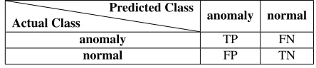
In the intrusion detection system, the most important performance measure is the accuracy of the detection, which means the classification ability of the neural network model. In order to evaluate the accuracy of the experiment, we introduce the concept of detection rate and false positive rate in the confusion matrix. The True Positive (TP) refers to the number of samples that the abnormal sample is identified as abnormal. The False Positive (FP) refers to the number of samples that the normal sample is identified as abnormal. The True Negative (TN) refers to the normal number of samples that the normal sample is identified as normal. The False Negative (FN) refers to the number of samples that the abnormal sample is identified as normal. Table 4 shows the definition of the confusion matrix. We have the following notation:
Accuracy (AC) is the percentage of the number of samples identified correctly over the total number of samples, as shown in Eq. (41).
AC = T P +T N
T P +T N+F P+F N (41)
True Positive Rate (TPR) is the percentage of the number of anomaly samples cor-rectly identified over the total number of anomaly samples, equal to the detection rate (DR), as shown in Eq.(42).
T P R= T P
T P +F N (42)
False Positive Rate (FPR) is the percentage of the number of normal samples erro-neously identified as anomaly samples over the total number of normal samples, as shown in Eq.(43).
F P R= F P
F P +T N (43)
Therefore, the goal of the intrusion detection system is to obtain a higher accuracy and detection rate with a lower false positive rate.
Table 4.Confusion matrix
Actual Class
Predicted Class
anomaly normal
anomaly TP FN
normal FP TN
6.4. Experiment Results and Discussion
categories: Normal, DoS, R2L, U2R, and Probe. In this experiment, KDDTrain+ is se-lected as the training dataset in NSL-KDD, and KDDTest-21 is sese-lected as the testing dataset.
In Section 6.2, we map 41-dimensional features to 122 dimensions, so the input layer of the neural network has 122 nodes. The output result is 5 categories, so the output layer of the neural network has 5 nodes. We set the number of the hidden layer nodes of the neural network as 80 nodes. At this point, the neural networks need 10245 parameters to be optimized, so the solution in IABC elite has a dimension of 10245. We set the population size of the bee colony as 100, the upper bound of the solution as 0.1, the lower bound as -0.1, and the maximum number of iterations of the IABC elite algorithm as 100. We select KDDTrain+ as the training dataset of BP neural network, and randomly take 30% of the data from it as a validation to avoid the BP neural network falling into overfitting. The cross-entropy is used as the error cost function of the backpropagation algorithm. In information theory, the cross entropy between two probability distributions over the same underlying set of events measures the average of bits needed to identify an event drawn from the set, if a coding scheme is used that is optimized for an ‘unnatural’ probability distribution, rather than the ‘true’ distribution. The average number of bits required for an event is also commonly used in error learning in machine learning. In order to speed up the neural network training process, the neural network is trained using the scaled conjugate gradient method [20].
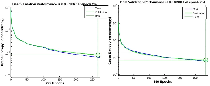
Fig. 5 shows the BPNN cross entropy error iteration curve for randomly generating neural network initial parameters for the BP neural network training. Fig. 6 shows the ABC BPNN cross entropy error iteration curve for the neural network training using the ABC algorithm pre-training parameters as initial parameters of the neural network. Fig. 7 shows the IABC elite BPNN cross entropy error iteration curve for the BP neural network training using the IABC elite algorithm pre-training parameters as initial parameters of the neural network. The experimental results show that the initial parameters generated by the pre-training of the IABC elite algorithm have lower initial errors, and the number of training epochs is smaller, which saves the time of neural network training.
0 50 100 150 200 250
10-3 10-2 10-1 100
Best Validation Performance is 0.0083867 at epoch 267
C ro s s -E n tr o p y (c ro s s e n tr o p y ) 273 Epochs Train Validation Best
Fig. 5.BPNN Error Cost Itera-tion Curve
0 50 100 150 200 250
10-3 10-2 10-1 100 101
Best Validation Performance is 0.0069011 at epoch 284
C ro s s -E n tr o p y (c ro s s e n tr o p y ) 290 Epochs Train Validation Best
Fig. 6. ABC BPNN Error Cost Iteration
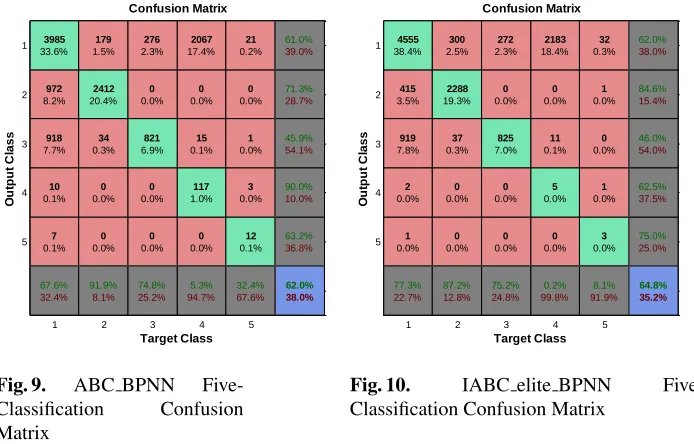
We test the neural network model on the KDDTest-21 testing dataset and use the five-classification confusion matrix to present the five-classification results. The class of labeling 1 in confusion matrix figure indicates the Normal class, the class of labeling 2 indicates the DoS class and the class of labeling 3 indicates the Probe class, the class of labeling 4 indicates the R2L class, and the class of labeling 5 indicates the U2R class. Fig. 8 is the classification result of five-classification confusion matrix of the neural network trained by a single BP algorithm. Fig. 9 is the classification result of five-classification confusion ma-trix of the neural network trained by BP algorithm optimized by ABC algorithm. Fig. 10 is the classification result of five-classification confusion matrix of the neural network trained by BP algorithm optimized by IABC elite algorithm. Overall, the total prediction accuracy in Fig. 9 is 1.4% higher than Fig. 8. The total prediction accuracy in Fig. 10 is 2.8% higher than Fig. 9. In the view of the Normal class, the classification accuracy predicted by the BP neural network optimized by IABC elite algorithm has been greatly improved, compared with the previous two figures. In the view of the five-classification confusion matrix, the BP neural networks optimized by IABC elite algorithm have better generalization ability.
0 20 40 60 80 100 120 140
10-3 10-2 10-1 100
Best Validation Performance is 0.01261 at epoch 138
C ro s s -E n tr o p y (c ro s s e n tr o p y ) 144 Epochs Train Validation Best
Fig. 7. IABC elite BPNN
Er-ror Cost Iteration Curve
1 2 3 4 5
1 2 3 4 5 3920 33.1% 948 8.0% 1001 8.4% 15 0.1% 8 0.1% 66.5% 33.5% 236 2.0% 2356 19.9% 33 0.3% 0 0.0% 0 0.0% 89.8% 10.2% 265 2.2% 0 0.0% 832 7.0% 0 0.0% 0 0.0% 75.8% 24.2% 2124 17.9% 0 0.0% 10 0.1% 64 0.5% 1 0.0% 2.9% 97.1% 21 0.2% 0 0.0% 1 0.0% 2 0.0% 13 0.1% 35.1% 64.9% 59.7% 40.3% 71.3% 28.7% 44.3% 55.7% 79.0% 21.0% 59.1% 40.9% 60.6% 39.4% Target Class O u tp u t C la s s Confusion Matrix
Fig. 8.BPNN Five-Classification Confusion Matrix
1 2 3 4 5 1 2 3 4 5 3985 33.6% 972 8.2% 918 7.7% 10 0.1% 7 0.1% 67.6% 32.4% 179 1.5% 2412 20.4% 34 0.3% 0 0.0% 0 0.0% 91.9% 8.1% 276 2.3% 0 0.0% 821 6.9% 0 0.0% 0 0.0% 74.8% 25.2% 2067 17.4% 0 0.0% 15 0.1% 117 1.0% 0 0.0% 5.3% 94.7% 21 0.2% 0 0.0% 1 0.0% 3 0.0% 12 0.1% 32.4% 67.6% 61.0% 39.0% 71.3% 28.7% 45.9% 54.1% 90.0% 10.0% 63.2% 36.8% 62.0% 38.0% Target Class O u tp u t C la s s Confusion Matrix
Fig. 9. ABC BPNN
Five-Classification Confusion Matrix
1 2 3 4 5
1 2 3 4 5 4555 38.4% 415 3.5% 919 7.8% 2 0.0% 1 0.0% 77.3% 22.7% 300 2.5% 2288 19.3% 37 0.3% 0 0.0% 0 0.0% 87.2% 12.8% 272 2.3% 0 0.0% 825 7.0% 0 0.0% 0 0.0% 75.2% 24.8% 2183 18.4% 0 0.0% 11 0.1% 5 0.0% 0 0.0% 0.2% 99.8% 32 0.3% 1 0.0% 0 0.0% 1 0.0% 3 0.0% 8.1% 91.9% 62.0% 38.0% 84.6% 15.4% 46.0% 54.0% 62.5% 37.5% 75.0% 25.0% 64.8% 35.2% Target Class O u tp u t C la s s Confusion Matrix
Fig. 10. IABC elite BPNN
Five-Classification Confusion Matrix
the optimum weight values and threshold values for Backpropagation algorithm. It make the Backpropagation algorithm find a better solution which have a better generalization performance in testing phase of the neural network. The IABC elite improved the con-vergence speed of the BP neural networks training and reduce the restrictions on initial weight values and threshold values, and avoid the neural network falling into a local op-timum. The simulation verify the effectiveness of intrusion detection systems based on IABC elite and BP neural networks.
7.
Conclusion
Acknowledgments.This work has been supported by the National Natural Science Foun-dation of China (No. 61672338 and No. 61873160).
References
1. Bullinaria, J.A., AlYahya, K.: Artificial bee colony training of neural networks. In: Nature Inspired Cooperative Strategies for Optimization (NICSO 2013), pp. 191–201. Springer (2014) 2. Cui, L., Li, G., Lin, Q., Du, Z., Gao, W., Chen, J., Lu, N.: A novel artificial bee colony algorithm with depth-first search framework and elite-guided search equation. Information Sciences 367, 1012–1044 (2016)
3. Cui, M., Han, D., Wang, J.: An efficient and safe road condition monitoring authentication scheme based on fog computing. IEEE Internet of Things Journal pp. 1–1 (2019)
4. Deng, Y.: What is the future of disk drives, death or rebirth? ACM Computing Surveys (CSUR) 43(3), 23 (2011)
5. Denning, D.E.: An intrusion-detection model. IEEE Transactions on software engineering 13(2), 222–232 (1987)
6. Du, Z., Liu, G., Bi, K., Jia, J., Han, D.: An improved artificial bee colony algorithm with elite-guided search equations. Computer Science & Information Systems 14(3) (2017)
7. Duda, R.O., Hart, P.E., Stork, D.G.: Pattern classification. John Wiley & Sons (2012) 8. Han, D., Bi, K., B., X., L., H., Wang, R.: An anomaly detection on the application-layer-based
qos in the cloud storage system. Computer Science & Information Systems 13(2) (2016) 9. Han, D., Bi, K., Liu, H., Jia, J.: A ddos attack detection system based on spark framework.
Computer Science & Information Systems 14(3) (2017)
10. Jaggi, R., Sangade, J.: Detecting and classifying attacks using artificial neural network. Int. J. Recent Innov. Trends Comput. Commun 2(5), 1136–1142 (2014)
11. Jiang, J., Wang, Z., Chen, T., Zhu, C., Chen, B.: Adaptive ap clustering algorithm and its appli-cation on intrusion detection. Journal on Communiappli-cations 36, 118–126 (2015)
12. Karaboga, D.: An idea based on honey bee swarm for numerical optimization. Tech. rep., Tech-nical report-tr06, Erciyes university, engineering faculty, Computer Engineering Department (2005)
13. Karaboga, D., Akay, B., Ozturk, C.: Artificial bee colony (abc) optimization algorithm for training feed-forward neural networks. In: Modeling Decisions for Artificial Intelligence. pp. 318–329. Springer Berlin Heidelberg (2007)
14. Karaboga, D., Basturk, B.: A powerful and efficient algorithm for numerical function optimiza-tion: artificial bee colony (abc) algorithm. Journal of Global Optimization 39(3), 459–471 (Nov 2007)
15. Karaboga, D., Basturk, B.: On the performance of artificial bee colony (abc) algorithm. Applied Soft Computing 8(1), 687–697 (2008)
16. Karaboga, D., Ozturk, C.: Neural networks training by artificial bee colony algorithm on pattern classification. Neural Network World 19(3), 279 (2009)
17. Kennedy, J.: Bare bones particle swarms. In: Proceedings of the 2003 IEEE Swarm Intelligence Symposium. SIS’03 (Cat. No. 03EX706). pp. 80–87. IEEE (2003)
18. Lee, W., Stolfo, S.J., Mok, K.W.: A data mining framework for building intrusion detection models. In: Proceedings of the 1999 IEEE Symposium on Security and Privacy (Cat. No. 99CB36344). pp. 120–132. IEEE (1999)
19. Lim, W.H., Isa, N.A.M.: An adaptive two-layer particle swarm optimization with elitist learning strategy. Information Sciences 273, 49–72 (2014)
21. Ozturk, C., Karaboga, D.: Hybrid artificial bee colony algorithm for neural network training. In: 2011 IEEE congress of evolutionary computation (CEC). pp. 84–88. IEEE (2011) 22. Qian, Q., Cai, J., Zhang, R.: Intrusion detection based on neural networks and artificial bee
colony algorithm. In: 2014 IEEE/ACIS 13th International Conference on Computer and Infor-mation Science (ICIS). pp. 257–262. IEEE (2014)
23. Qiu, C., Shan, J., Shandong, B., et al.: Research on intrusion detection algorithm based on bp neural network. International Journal of Security and its Applications 9(4), 247–258 (2015) 24. Revathi, S., Malathi, A.: A detailed analysis on nsl-kdd dataset using various machine learning
techniques for intrusion detection. International Journal of Engineering Research & Technol-ogy (IJERT) 2(12), 1848–1853 (2013)
25. SHEN Xiajiong, WANG Long, H.D.: Application of bp neural network optimized by artificial bee colony in intrusion detection. Computer Engineering 42(2), 190 (2016)
26. Tavallaee, M., Bagheri, E., Lu, W., Ghorbani, A.A.: A detailed analysis of the kdd cup 99 data set. In: 2009 IEEE Symposium on Computational Intelligence for Security and Defense Applications. pp. 1–6. IEEE (2009)
27. Wang, H., Wu, Z., Rahnamayan, S., Sun, H., Liu, Y., Pan, J.s.: Multi-strategy ensemble artificial bee colony algorithm. Information Sciences 279, 587–603 (2014)
28. Xie, J., Deng, Y., Min, G., Zhou, Y.: An incrementally scalable and cost-efficient interconnec-tion structure for data centers. IEEE Transacinterconnec-tions on Parallel and Distributed Systems 28(6), 1578–1592 (2017)
29. Yao, X.: Evolutionary artificial neural networks. International journal of neural systems 4(03), 203–222 (1993)
30. Yao, X., Islam, M.M.: Evolving artificial neural network ensembles. IEEE Computational In-telligence Magazine 3(1), 31–42 (2008)
31. Yin, C., Zhu, Y., Fei, J., He, X.: A deep learning approach for intrusion detection using recurrent neural networks. IEEE Access 5, 21954–21961 (2017)
32. Zhu, G., Kwong, S.: Gbest-guided artificial bee colony algorithm for numerical function opti-mization. Applied mathematics and computation 217(7), 3166–3173 (2010)
Letian Duanis currently a master student of Shanghai Maritime University. His research interests include cloud computing and Big Data.
Dezhi Hanreceived the Ph.D. degree from the Huazhong University of Science and Tech-nology. He is currently a Professor of computer science and engineering with Shanghai Maritime University. His research interests include cloud computing, mobile networking, wireless communication, and cloud security.
Qiuting Tian is currently a Ph.D. candidate at Shanghai Maritime University. Her re-search interests include cloud computing, mobile networking security and cloud security.