Intelligent System Stability using Type-2 Fuzzy Controller

(1)

penerbit.uthm.edu.my/ojs/index.php/ijie

Abstract: To avoid mathematical complexity, Interval T2FSs (IT2FSs) have been pertained in majority of the fields. Type-2 fuzzy sets (T2FSs) handle a greater modeling and uncertainties that exist in the real world applications especially in control systems. One of the important components that influence the fuzzy controller is the triangular norm, which is the aggregation operator. For getting the stability of a control system T-norm operator can be preferred. Gaussian Interval Type-2 Membership Function (GIT2MF) has been used in this research. Mathematical properties of aggregation operator also proved using Gaussian Interval Type-2 Weighted Arithmetic (GIT2WA) operator. The aim of this research is analyzing the stability of an inverted pendulum using Interval Type-2 Fuzzy Logic Controller (IT2FLC) and the results are compared with traditional Proportional Integrated Derivative (PID) controller. It is observed that IT2FL controller gives better stability under imprecise condition.

Keywords: Gaussian membership function, T-norm, type-2 fuzzy sets, PID controllers, interval type-2 fuzzy logic controller, inverted pendulum, stability analysis.

INTERNATIONAL JOURNAL OF INTEGRATED ENGINEERING VOL. 11 NO. 1 (2019) 270-282

IJIE

Journal homepage: http://penerbit.uthm.edu.my/ojs/index.php/ijie ISSN : 2229-838X e-ISSN : 2600-7916

The International

Journal of

Integrated

Engineering

Intelligent System Stability using Type-2 Fuzzy Controller

D. Nagarajan

1

, J. Kavikumar

2,*

, M. Lathamaheswari

1

, S. Broumi

3

1_{Department of Mathematics, Hindustan Institute of Technology & Science, Chennai, 603103, INDIA}

2_{Faculty of Applied Sciences & Technology, Universiti Tun Hussein Onn Malaysia, Parit Raja, Johor, 86400,}

MALAYSIA

3_{Laboratory of Information Processing Faculty of Science Ben M’Sik, University Hassan II, Casablanca, MOROCCO}

*Corresponding Author

DOI: https://doi.org/10.30880/ijie.2019.11.01.027

Received 11 October 2018; Accepted 28 February 2019; Available online 30 April 2019

1. Introduction

Fuzzy Control Systems (FCSs) is an abstraction of the human maturity for using linguistic rules with vague implication in order to develop control behavior [1]. A triangular norm plays an important role in Control systems. Fuzzy Logic Controller (FLC) consists of linguistic IF-THEN rules. In the comparison of Type1 (T1) and Type-2 (T2) categories in FL, T1FL system has the difficulties in emulate and curtail the effect of uncertainties, due to its certainty i.e., for every input there is a crisp membership grade. While in the case of T2 Fuzzy Logic Systems, at least one T2FS must be taken which should be characterized by membership grades which independently fuzzy. This case is useful in situations where the difficulties are concluded the exact membership grades and this would be useful to handle such cases, also it has the possibility to outperform their T1 counterparts. To disciple T2 fuzzy output sets into T1, a type reducer is needed and therefore the defuzzifier for giving precise output can develop them. Moreover in IT2FSs, every element of footprint of uncertainity (FOU) has a unity secondary membership grade. Under fuzzy based control design, membership functions and rule base are the important things and it is difficult to determine. In this work, to construct the antecedents of the rule base IT2FS is used, to handle uncertainties, whereas for consequents T1FS is applied. Type reduction process is differentiate T2 from T1 since for each fired rules the outputs are T2FS and this should be done prior to the defuzzifier is manipulate to provoke an output in a crisp manner. Center of sets can be the type reducer. This will incorporate each and every T2 outputs and produce T1 set, which is the type reduced set. It has been noted

*Corresponding author: [email protected]

(2)

that Interval T2FL controllers are applied in control of, the mobile robot quality, sound speakers and admission in ATM networks [2].

FL controllers are regularly designed by T1FS, which is known as T1FL controllers, and it has been applied in many of the fields, specifically in controlling complex non-linear systems and the researchers faced the difficulties in modelling and handling uncertainties. The disadvantage of this model is failing to seize all the feature of a certain plant. Generally, controllers which will handles more uncertainties are preferable. Since MF virtually expresses the fuzziness, its characterization is the main aspect of the fuzzy operation [3]. The most applicable membership functions in control applications are Triangular and Trapezoidal. Since these MFs are producing poor approximations, Gaussian Membership Function (GMF) is chosen as it gives actual representation at each point. In fuzzy inference theory, MFs, Triangular norm operators, defuzzification methods and input types to the controller are the main components. The selection of T Norm, defuzzifier and GMF has the greatest influence of the fuzzy controller [4]. Classical control designs are based on point to point whereas FL controller is either range to point or range to range i.e. FL controller is a function from an input data vector to a scalar output [5, 6]. In this work, GIT2MF with uncertain mean and standard deviation is considered. In the case of T2FS, the antecedent and consequent parts are T2 or any one of the two. Usually consequent part is taken as T1 ([7, 8, 9, 10, 11]. The FOU processes the stability analysis of the system [12, 13, 14]. Input components will affect the stability of the system. Hence to maintain the stability of the systems inputs have to be monitored in a regular manner [15, 16, 17, 18, 19].

2. Illustrations

2.1 Gaussian Membership Function

Gaussian membership function for a fuzzy set is defined by 𝜓̅(𝑥) = 𝑒𝑥𝑝 [− 1 (𝑥−𝑚)] , −∞ < 𝑥 < ∞, where 𝑚 is

the mean and 𝜎 is the standard deviation.

𝐷 ₂ _𝜎

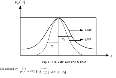
2.2 Gaussian Membership Function with Type-2 Fuzzy Set

Here two different cases are considered for GITMF according to the nature of the parameters, mean (𝑚) and standard deviation (𝜎) namely GIT2MF with fixed mean and uncertain standard deviation (FM & USD) and fixed standard deviation and uncertain mean (FSD & UM) as follows:



_D



x



 



1

x

Fig. 1 – GIT2MF with FM & USD

and it is defined by ( ) 1 𝑥−𝑚 2 𝜓𝐷̅ 𝑥 = 𝑒𝑥𝑝 [− (

2 _𝜎) ] , 𝜎 ∈ [𝜎1, 𝜎2]



₁

LMF



2

(3)

(4)



_D



x



  

1

x

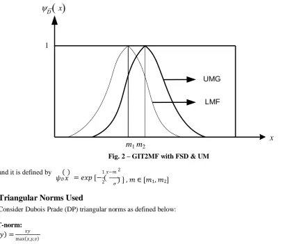
Fig. 2 – GIT2MF with FSD & UM

and it is defined by ( ) 1 𝑥−𝑚 2 𝜓𝐷̅ 𝑥 = 𝑒𝑥𝑝 [− (

2 _𝜎) ] , 𝑚 ∈ [𝑚1, 𝑚2]

2.3 Triangular Norms Used

Consider Dubois Prade (DP) triangular norms as defined below:

DP T-norm:

𝑇(𝑥, 𝑦) = 𝑥𝑦

max(𝑥,𝑦,𝑣) (1)

DP T-conorm:

𝑇𝐶(𝑥, 𝑦) = 1 − [ (1−𝑥)(1−𝑦) ] (2)

max[(1−𝑥),(1−𝑦),(1−𝑣)]

In this paper, T-norm is used as it is preferable for control systems with min and max operations and T-conorm will be used in the stage of defuzzification in the control system with uncertain parameters.

3. Operational Laws

Let 𝐷̅, 𝐷̅1, 𝐷̅2 be three Gaussian Interval Type-2 Fuzzy Numbers and 𝜗 ∈ [0,1] then the following operations are hold.

Addition Operation:

1 𝑥1−𝑚1 2 1 𝑥2−𝑚2 2

𝐷̅ ⊕ 𝐷̅

= 1 − [ (1−𝑒𝑥𝑝[−2( 𝜎1 ) ])(1−𝑒𝑥𝑝[−2( 𝜎2 ) ]) ] (3)

1 2

1 𝑥1−𝑚1 2 1 𝑥2−𝑚2 2 ₍ ₎

𝑚𝑎𝑥((1−𝑒𝑥𝑝[−₂(

𝜎1 ) ]),(1−𝑒𝑥𝑝[−2( 𝜎2 ) ]), 1−𝜗 )

Multiplication Operation:

1 𝑥1−𝑚1 2 1 𝑥2−𝑚2 2

(𝑒𝑥𝑝[− ( ) ])(𝑒𝑥𝑝[− ( ) ])

𝐷̅ ⊗ 𝐷̅ = 1 − [ 2 𝜎1 2 𝜎2 _] ₍₄₎

1 2

1 𝑥1−𝑚1 2 1 𝑥2−𝑚2 2

𝑚𝑎𝑥((𝑒𝑥𝑝[−₂(

𝜎1 ) ]),(𝑒𝑥𝑝[−2( 𝜎2 ) ]),𝜗)

Multiplication by an ordinary number and Power:

1 𝑥−𝑚 2 𝑡

𝑡. 𝐷̅ = 1 −

(1−𝑒𝑥𝑝[− (

2 𝜎 ) ] )

(5)

1 𝑥−𝑚 2 𝑡

max((1−𝑒𝑥𝑝[−₂( _𝜎) ] ),(1−𝜗))

[ ]

m

₁

m

₂

(5)

Nagarajan et al., Int. J. of Integrated Engineering Vol. 11 No. 1 (2019) p. 270-282

273

and

1 𝑥−𝑚 2 𝑡

𝐷̅𝑡 ₌ (𝑒𝑥𝑝[− ( 2 𝜎 ) ] )

(6)

1 𝑥−𝑚 2 𝑡

max((𝑒𝑥𝑝[− (

[ 2 𝜎 ) ] ),𝜗) ]

4. Proposed Theorems

The below theorems are constituting the mathematical properties of aggregation operator (AO) namely triangular norms and shows the role of their properties in the control system. Here the theorems of first, Idempotency, associativity and stability represent the facts that a control system can have any number of inputs (finite), unanimity of the system, the system can extend the process without ambiguity and the strength of the system respectively.

Theorem 4.1: Let ̅ 1 𝑥𝑖−𝑚𝑖 2 be a collection of GIT2FNs then their aggregated value by

𝐷𝑖 = (𝑒𝑥𝑝 [− ₂( 𝜎𝑖 ) ]) , 𝑖 = 1,2, ⋯ , 𝑛

GIT2WG operator is still a GIT2FN and

1 𝑥 −𝑚 2 𝜔̅̅ 𝑖

𝑀𝑂𝑇(1−𝑒𝑥𝑝[− ( 𝑖 𝑖) ])

𝐺𝐼𝑇2𝑊𝐴 (𝐷̅ , 𝐷̅ , ⋯ , 𝐷̅ ) = 1 − 2 𝜎𝑖

𝜔̅̅ 1 2 𝑛

1 𝑥1−𝑚1 2 𝜔̅̅ 1 1 𝑥2−𝑚2 2 𝜔̅̅ 2 1 𝑥𝑛−𝑚𝑛 2 𝜔̅̅ 𝑛 ( )

𝑚𝑎𝑥((1−𝑒𝑥𝑝[−₂(

𝜎1 ) ]) ,(1−𝑒𝑥𝑝[−2( 𝜎2 ) ]) ,⋯,(1−𝑒𝑥𝑝[−2( 𝜎𝑛 ) ]) , 1−𝜗 )

(7)

where 𝑀𝑂𝑇 is Multiplication Of Terms.

Proof:

By the method of mathematical induction. For 𝑛 = 2, using the law of multiplication by an ordinary number,

𝜔̅̅ . 𝐷̅ = 1 −

1 𝑥−𝑚 2

(1−𝑒𝑥𝑝[−₂( _𝜎) ])

𝜔̅̅ 1

.

1

1 𝑥−𝑚 2 𝜔̅̅ 𝑖 ( )

𝑚𝑎𝑥((1−𝑒𝑥𝑝[− ( ) ]) , 1−𝜗 )

[ 2 𝜎 ]

1 𝑥 −𝑚 2 𝜔̅̅ 𝑖

𝑀𝑂𝑇(1−𝑒𝑥𝑝[− ( 𝑖 𝑖) ])

Now, for 𝑖 = 1,2. 𝐺𝐼𝑇2𝑊𝐴 (𝐷̅ , 𝐷̅ ) = 1 − 2 𝜎𝑖

,

𝜔̅̅ 1 2 _{1 𝑥1−𝑚1 2} 𝜔̅̅ 1 1 𝑥2−𝑚2 2 𝜔̅̅ 2

𝑚𝑎𝑥((1−𝑒𝑥𝑝[− (

2 𝜎1 ) ]) ,(1−𝑒𝑥𝑝[− ( 2 𝜎2 ) ]) ,(1−𝜗))

1 𝑥𝑖−𝑚𝑖 2𝜔̅̅ 𝑖

̅ ̅ 𝑀𝑂𝑇(1−𝑒𝑥𝑝[−2( 𝜎𝑖 ) ])

𝐺𝐼𝑇2𝑊𝐴𝜔̅̅ (𝐷1, 𝐷2) = 1 − 1 𝑥 −𝑚 2𝜔̅̅ 1 1 𝑥 −𝑚 2𝜔̅̅ 2 .

𝑚𝑎𝑥((1−𝑒𝑥𝑝[− ( 1 1) ]),(1−𝑒𝑥𝑝[− ( 2 2) ]),(1−𝜗))

2 𝜎1 2 𝜎2

For 𝑛 = 𝑘,

𝟏 𝒙 −𝒎 𝟐 𝝎̅ 𝒊

𝑴𝑶𝑻(𝟏−𝒆𝒙𝒑[− ( 𝒊 𝒊) ]) 𝑮𝑰𝑻𝟐𝑾𝑨 𝝎̅ (𝑫̅ 𝟏, 𝑫̅ 𝟐, ⋯ , 𝑫̅ 𝒌) = 𝟏 −

𝟏 𝒙𝟏−𝒎𝟏 𝟐 𝝎̅ 𝟏

𝟐

𝟏 𝒙𝟐−𝒎𝟐 𝝈𝒊

𝟐 𝝎̅ 𝟐 _{𝟏 𝒙𝒌−𝒎𝒌}𝟐 𝝎̅ 𝒌 ₍ ₎.

For 𝑛 = 𝑘 + 1,

𝒎𝒂𝒙((𝟏−𝒆𝒙𝒑[− (

(6)

𝑖 𝑖 𝑖

𝐺𝐼𝑇2𝑊𝐴𝜔̅̅ (𝐷̅1, 𝐷̅2, ⋯ , 𝐷̅𝑘, 𝐷̅𝑘+1) = 1 −

1 𝑥 −𝑚 2 𝜔̅̅ 𝑖

𝑀𝑂𝑇(1−𝑒𝑥𝑝[− ( 𝑖 𝑖) ])

2 𝜎𝑖 _{⊗ 1 −}

1 𝑥 −𝑚 2 𝜔̅̅ 1 1 𝑥 −𝑚 2 𝜔̅̅ 2 1 𝑥 −𝑚 2 𝜔̅̅ 𝑘

𝑚𝑎𝑥((1−𝑒𝑥𝑝[− ( 1 1) ]) ,(1−𝑒𝑥𝑝[− ( 2 2) ]) ,⋯,(1−𝑒𝑥𝑝[− ( 𝑘 𝑘) ]) , (1−𝜗))

2 𝜎1

1 𝑥 −𝑚

2 𝜎2

2 𝜔̅̅ 𝑘+1

2 𝜎𝑘

(1−𝑒𝑥𝑝[− ( 𝑘+1 𝑘+1) ])

2

1 𝑥 𝜎𝑘+1

−𝑚 2 𝜔̅̅ 𝑘+1

𝑚𝑎𝑥( (1−𝑒𝑥𝑝[− ( 𝑘+1 𝑘+1) ]) ,(1−𝜗))

2 _𝜎𝑘+1

1 𝑥 −𝑚 2 𝜔̅̅ 𝑖

𝑀𝑂𝑇(1−𝑒𝑥𝑝[− ( 𝑖 𝑖) ])

= 1 − _{1 𝑥 −𝑚 2} _{𝜔̅̅ 1} _{1 𝑥 −𝑚 2}2 _{𝜔̅̅ 2}𝜎𝑖 _{1 𝑥} _−𝑚 2 𝜔̅̅ 𝑘+1 .

𝑚𝑎𝑥((1−𝑒𝑥𝑝[− ( 1 1) ]) ,(1−𝑒𝑥𝑝[− ( 2 2) ]) ,⋯,(1−𝑒𝑥𝑝[− ( 𝑘+1 𝑘+1) ]) , (1−𝜗))

2 𝜎1 2 𝜎2 2 _𝜎𝑘+1

Hence (1) is true for all the values of 𝑛.

Theorem 4.2: (Idempotency) Let ̅ 1 𝑥𝑖−𝑚𝑖 2 be a collection of GIT2FNs. If for all

𝐷𝑖 = (𝑒𝑥𝑝 [− ₂( 𝜎𝑖 ) ]) , 𝑖 = 1,2, ⋯ , 𝑛

𝐷̅_𝑖, 𝑖 = 1,2, ⋯ , 𝑛 are equal i.e., 𝐷̅_𝑖= 𝐷̅ _then𝐺𝐼𝑇2𝑊𝐴𝜔̅̅ (𝐷̅1, 𝐷̅2, … , 𝐷̅𝑛) = 𝐷̅.

Proof: Using theorem 4.1,

1 𝑥 −𝑚 2 𝜔̅̅ 𝑖

𝑀𝑂𝑇(1−𝑒𝑥𝑝[− ( 𝑖 𝑖) ])

𝐺𝐼𝑇2𝑊𝐴 (𝐷̅ , 𝐷̅ , ⋯ , 𝐷̅ ) = 1 − 2 𝜎𝑖

𝜔̅̅ 1 2 𝑛 _{1 𝑥1−𝑚1 2} 𝜔̅̅ 1 1 𝑥2−𝑚2 2 𝜔̅̅ 2 1 𝑥𝑛−𝑚𝑛 2 𝜔̅̅ 𝑛

2 𝜎1 ) ]) ,(1−𝑒𝑥𝑝[− ( 2 𝜎2 ) ]) ,⋯,(1−𝑒𝑥𝑝[− ( 2 𝜎𝑛 ) ]) , (1−𝜗))

1 𝑥 −𝑚

𝑀𝑂𝑇(1−𝑒𝑥𝑝[− ( ) ]) 2 ∑𝑛 𝜔̅̅ 𝑖

𝐺𝐼𝑇2𝑊𝐴 (𝐷̅ , 𝐷̅ , ⋯ , 𝐷̅ ) = 1 − 2 𝜎𝑖

𝜔̅̅ 1 2 𝑛 _{1 𝑥1−𝑚1 2} 𝜔̅̅ 1 1 𝑥2−𝑚2 2 𝜔̅̅ 2 1 𝑥𝑛−𝑚𝑛 2 𝜔̅̅ 𝑛

2 𝜎1 ) ]) ,(1−𝑒𝑥𝑝[− ( 2 𝜎2 ) ]) ,⋯,(1−𝑒𝑥𝑝[− ( 2 𝜎𝑛 ) ]) , (1−𝜗))

1 𝑥𝑖−𝑚𝑖 2

𝐺𝐼𝑇2𝑊𝐴 (𝐷̅ , 𝐷̅ , ⋯ , 𝐷̅ ) = 1 − 𝑀𝑂𝑇(1−𝑒𝑥𝑝[− ( 2 𝜎𝑖 ) ]) = 𝐷̅.

𝜔̅̅ 1 2 𝑛 1 𝑥1−𝑚1 2 1 𝑥2−𝑚2 2 1 𝑥𝑛−𝑚𝑛 2 ₍ ₎

2 𝜎1 ) ]), (1−𝑒𝑥𝑝[−2( 𝜎2 ) ]),⋯,(1−𝑒𝑥𝑝[− ( 2 𝜎𝑛 ) ]), 1−𝜗 )

Theorem 4.3: (Associativity)

If

𝐷̅1, 𝐷̅2 and 𝐷̅3 are the three GIT2FNs then the following result (𝐷̅1 ⊕ 𝐷̅2 ⊕ 𝐷̅3) = (𝐷̅1 ⊕ 𝐷̅2) ⊕ 𝐷̅3 is hold.

Proof: Using associativity property we have (𝐷̅₁_{⊕ 𝐷}̅₂_{⊕ 𝐷}₃̅ _{) = (𝐷}̅₁_{⊕ 𝐷}̅₂_{) ⊕ 𝐷}̅₃_{. Consider,}

(𝐷̅ ⊕ 𝐷̅ ) ̅ 1 𝑥1−𝑚1 2 1 𝑥2−𝑚2 2 1 𝑥3−𝑚3 2

1 2 ⊕ 𝐷3 = [(1 − 𝑒𝑥𝑝 [− ₂( 𝜎1 ) ]) ⊕ (1 − 𝑒𝑥𝑝 [− ( 2 𝜎2 ) ])] ⊕ (1 − 𝑒𝑥𝑝 [− ( 2 𝜎3 ) ])

1 𝑥1−𝑚1 2 1 𝑥2−𝑚2 2 1 𝑥3−𝑚3 2

= 1 − [(1−𝑒𝑥𝑝[−21 𝑥1−𝑚1 2 ( 𝜎1 ) ])⊕(1−𝑒𝑥𝑝[−2( 1 𝑥2−𝑚2 2 𝜎2 ) ])] ̇(1−𝑒𝑥𝑝[−2( 1 𝑥3−𝑚3 2 𝜎3 ) ])

max[[(1−𝑒𝑥𝑝[−₂(

𝜎1 ) ])⊕(1−𝑒𝑥𝑝[−2(

1 𝑥1−𝑚1 2 𝜎2 1 𝑥2−𝑚2 2 ) ])](1−𝑒𝑥𝑝[−2( 𝜎3 ) ]),(1−𝜗)]

(1−𝑒𝑥𝑝[− ( ) ]) ̇(1−𝑒𝑥𝑝[− ( _{) ])}

2

1− 2 𝜎1 2 𝜎2 1 𝑥3−𝑚3

1 𝑥̇1−𝑚1 2 1 𝑥2−𝑚2 2 ̇(1−𝑒𝑥𝑝[− ( 2 𝜎3 ) ])

max[(1−𝑒𝑥𝑝[− ( ₂

= 𝜎1 2 ) ]), (1−𝑒𝑥𝑝[− ( 2 𝜎2 ) ]), (1−𝜗)] 2

1 𝑥1−𝑚1 1 𝑥2−𝑚2

max[ (1−𝑒𝑥𝑝[− ( ₂ 𝜎1 ) ]) ̇ (1−𝑒𝑥𝑝[− ( ₂ 𝜎2 ) ]) 1 𝑥3−𝑚3 2

1 𝑥1−𝑚1 2 1 𝑥2−𝑚2 2 , (1−𝑒𝑥𝑝[− ( 2 𝜎3 ) ]),(1−𝜗)]

max[(1−𝑒𝑥𝑝[− (

2 𝜎1 ) ]), (1−𝑒𝑥𝑝[− ( 2 𝜎2 ) ]), (1−𝜗)]

= 𝐷̅1 ⋅𝐷̅2⋅𝐷̅3

max[𝐷̅ ,𝐷̅ ,(1−𝜗)] max[ 𝐷̅ 1⋅𝐷̅ 2 _,𝐷_{̅ ,(1−𝜗)]}

1 2 _max[𝐷_{̅ 1,𝐷}_{̅ 2,(1−𝜗)] 3}

1 𝑥1−𝑚1 2 1 𝑥2−𝑚2 2 1 𝑥3−𝑚3 2

(1−𝑒𝑥𝑝[− ( ) ]) ̇(1−𝑒𝑥𝑝[− ( ) ]) ̇(1−𝑒𝑥𝑝[− ( ) ]) = 1 − 2 _{1 𝑥1−𝑚1 2}𝜎1 _{1 𝑥2−𝑚2 2}2 𝜎2 _{1 𝑥3−𝑚3 2}2 𝜎3

max[(1−𝑒𝑥𝑝[− (

(7)

275

2

= 1 − 𝐷̅1 ⋅𝐷̅2⋅𝐷̅3 _{= (𝐷}_{̅ ⊕ 𝐷̅ ⊕ 𝐷̅ )}.

max[𝐷̅₁,𝐷̅₂,𝐷̅₃,(1−𝜗)] 1 2 3

This result also holds for all the values of 𝑛.

Theorem 4.4: (Stability) Let ̅ 1 𝑥𝑖−𝑚𝑖 2 _{be a collection of GIT2FNs. If}𝑝 > 0 _and

𝐷̅ 1 𝑥𝑛+1−𝑚𝑛+1

𝐷𝑖 = (𝑒𝑥𝑝 [− ₂(

2 𝜎𝑖

) ]) , 𝑖 = 1,2, ⋯ , 𝑛

𝑛+1 = (𝑒𝑥𝑝 [− ₂( 𝜎𝑛+1 ) ]) is a GIT2FN on the set 𝑋 then

𝐺𝐼𝑇2𝑊𝐴𝜔̅̅ (𝑝 ⋅ 𝐷̅1 ⊕ 𝐷̅𝑛+1, 𝑝 ⋅ 𝐷̅2 ⊕ 𝐷̅𝑛+1, ⋯ , 𝑝 ⋅ 𝐷̅𝑛 ⊕ 𝐷̅𝑛+1) = 𝑝 ⋅ [𝐺𝐼𝑇2𝑊𝐴𝜔̅̅ (𝐷̅1, 𝐷̅2, ⋯ , 𝐷̅𝑛)] ⊕ 𝐷̅𝑛+1.

1 𝑥−𝑚 2 𝑝

Proof: Using power operation of GIT2FN,. 𝐷̅ = 1 − [ (1−𝑒𝑥𝑝[− ( 2 𝜎 ) ]) ]_.

1 𝑥−𝑚 2 𝑝

2 𝜎 ) ]) ,(1−𝜗))

We know that, 𝐺𝐼𝑇2𝑊𝐴𝜔̅̅ (𝐷̅1 ⊕ 𝐷n+1̅ , 𝐷̅2 ⊕ 𝐷̅n+1, ⋯ , 𝐷̅𝑛 ⊕ 𝐷̅n+1) = 𝐺𝐼𝑇2𝑊𝐴𝜔̅̅ (𝐷̅1, 𝐷̅2, ⋯ , 𝐷̅𝑛) ⊕ 𝐷̅n+1 (8)

𝑀𝑂𝑇𝑛+1

𝑝

1 𝑥 𝑗−𝑚𝑗

Now, 𝐺𝐼𝑇2𝑊𝐴 (𝐷̅ ⊕ 𝐷̅ ) = 1 − 𝑗=1 (1−𝑒𝑥𝑝[− ( 𝜎𝑗 ) ])

𝜔̅̅ i n+1 𝑝

1 𝑥𝑗−𝑚𝑗

( ) max[(1−𝑒𝑥𝑝[− (

2 𝜎𝑗 ) ]) , 1−𝜗 ]

𝐺𝐼𝑇2𝑊𝐴𝜔̅̅ (𝑝 ⋅ 𝐷̅1 ⊕ 𝐷̅𝑛+1, 𝑝 ⋅ 𝐷̅2 ⊕ 𝐷̅𝑛+1, ⋯ , 𝑝 ⋅ 𝐷̅𝑛 ⊕ 𝐷̅𝑛+1)

𝑀𝑂𝑇𝑛+1 1 𝑥𝑗−𝑚𝑗 2 𝜔̅̅ 𝑗 1 𝑥𝑛+1−𝑚𝑛+1 2

= 1 − 𝑗=1 (1−𝑒𝑥𝑝[−2( _𝜎𝑗) ]) 𝜔̅̅

(1−𝑒𝑥𝑝[− (

2 _𝜎𝑛+1 ) ])

(9)

1 𝑥𝑗−𝑚𝑗 2 𝑗 1 𝑥 −𝑚 2

max[(1−𝑒𝑥𝑝[− ( ) ])

,(1−𝑒𝑥𝑝[− ( 𝑛+1 𝑛+1) ]),(1−𝜗)]

2 𝜎𝑗 2 𝜎𝑛+1

𝐺𝐼𝑇2𝑊𝐴𝜔̅̅ (𝐷̅1, 𝐷̅2, ⋯ , 𝐷̅𝑛) ⊕ 𝐷̅𝑛+1 =

𝑀𝑂𝑇𝑛 1 𝑥𝑗−𝑚𝑗 2 𝜔̅̅ 𝑗

𝑗=1(1−𝑒𝑥𝑝[− (

𝜎𝑗 ) ]) 1 𝑥 −𝑚 2

1 −

1 𝑥1−𝑚1 2 𝜔̅̅ 1 1 𝑥2−𝑚2 2 𝜔̅̅ 2 1 𝑥𝑛−𝑚𝑛 2 𝜔̅̅ 𝑛 ⊕ (1 − 𝑒𝑥𝑝 [− 2 (

𝑛+1 𝑛+1_{) ])}

𝜎𝑛+1

max((1−𝑒𝑥𝑝[− (

2 𝜎1 ) ]) ,(1−𝑒𝑥𝑝[− ( 2 𝜎2 ) ]) ,⋯,(1−𝑒𝑥𝑝[− ( 2 𝜎𝑛 ) ]) , (1−𝜗))

𝑀𝑂𝑇𝑛 1 𝑥𝑗−𝑚𝑗 2 𝜔̅̅ 𝑗 1 𝑥𝑛+1−𝑚𝑛+1 2

= 1 − 𝑗=1(1−𝑒𝑥𝑝[−2( _𝜎𝑗) ]) ⋅(1−𝑒𝑥𝑝[− ( 2 _𝜎𝑛+1 ) ])

(10)

𝑥 −𝑚 2 𝜔̅̅ 𝑗 ₂

max(𝑀𝑂𝑇𝑛 1 𝑗 𝑗_{) ])} 1 𝑥𝑛+1−𝑚𝑛+1) ]), (1−𝜗))

𝑗=1[(1−𝑒𝑥𝑝[− ( _𝜎𝑗 ],(1−𝑒𝑥𝑝[−₂( 𝜎𝑛+1

From (9) and (10),

𝐺𝐼𝑇2𝑊𝐴𝜔̅̅ (𝐷̅1 ⊕ 𝐷̅𝑛+1, 𝐷̅2 ⊕ 𝐷̅𝑛+1, ⋯ , 𝐷̅𝑛 ⊕ 𝐷̅𝑛+1) = 𝐺𝐼𝑇2𝑊𝐴𝜔̅̅ (𝐷̅1, 𝐷̅2, ⋯ , 𝐷̅𝑛) ⊕ 𝐷̅𝑛+1.

Also we have, 𝐺𝐼𝑇2𝑊𝐴𝜔̅̅ (𝑝. 𝐷̅1, 𝑝. 𝐷̅2, ⋯ , 𝑝. 𝐷̅𝑛) = 𝑝. (𝐺𝐼𝑇2𝑊𝐴𝜔̅̅ (𝐷̅1, 𝐷̅2, ⋯ , 𝐷̅𝑛)). (11)

𝐺𝐼𝑇2𝑊𝐴𝜔̅̅ (𝑝. 𝐷̅1, 𝑝. 𝐷̅2, ⋯ , 𝑝. 𝐷̅𝑛)

𝑀𝑂𝑇𝑛 1 𝑥𝑗−𝑚𝑗 2 𝑝

𝜔̅̅ 𝑗

𝑗=1(1−𝑒𝑥𝑝[− ( _𝜎𝑗 ) ] )

= 1 −

1 𝑥1−𝑚1 2 𝑝 𝜔̅̅ 1 1 𝑥2−𝑚2 2 𝑝 𝜔̅̅ 2 1 𝑥𝑛−𝑚𝑛 2 𝑝 𝜔̅̅ 𝑛 ₍ ₎

max((1−𝑒𝑥𝑝[−₂(

𝜎1 ) ] )

,(1−𝑒𝑥𝑝[− (

2

𝑀𝑂𝑇𝑛

𝜎2 ) ] )

1 𝑥𝑗−𝑚𝑗

,⋯,(1−𝑒𝑥𝑝[− (

2

2 𝑝𝜔̅̅ 𝑗

𝜎𝑛 ) ] ) , 1−𝜗 )

= 1 − 𝑗=1(1−𝑒𝑥𝑝[−2( 𝜎𝑗 ) ] ) (12)

1 𝑥1−𝑚1 2 𝑝𝜔̅̅ 1 1 𝑥2−𝑚2 2 𝑝𝜔̅̅ 2 1 𝑥𝑛−𝑚𝑛 2 𝑝𝜔̅̅ 𝑛

Also, since

𝜎1 ) ]

),(1−𝑒𝑥𝑝[− (

2 _𝜎2) ] ),⋯,(1−𝑒𝑥𝑝[− ( 2 _𝜎𝑛) ] ), (1−𝜗))

𝑝. (𝐺𝐼𝑇2𝑊𝐴𝜔̅̅ (𝐷̅1, 𝐷̅2, ⋯ , 𝐷̅𝑛))

𝑀𝑂𝑇𝑛 1 𝑥𝑗−𝑚𝑗 2 𝜔̅̅ 𝑗

𝑝

= 1 − 𝑗=1

(1−𝑒𝑥𝑝[− (

𝑝

) ] )

𝜎𝑗

𝑝 𝑝

1 𝑥1−𝑚1 2 𝜔̅̅ 1 1 𝑥2−𝑚2 2 𝜔̅̅ 2 1 𝑥𝑛−𝑚𝑛 2 𝜔̅̅ 𝑛

𝜎1 ) ]

) ,(1−𝑒𝑥𝑝[− (

2 _𝜎2) ] ) ,⋯,(1−𝑒𝑥𝑝[− ( 2 _𝜎𝑛) ] ) , (1−𝜗))

(8)

𝑀𝑂𝑇𝑛 1 𝑥𝑗−𝑚𝑗 2 𝑝𝜔̅̅ 𝑗

= 1 − 𝑗=1

(1−𝑒𝑥𝑝[−₂(

𝜎𝑗 ) ] )

(13)

1 𝑥1−𝑚1 2 𝑝𝜔̅̅ 1 1 𝑥2−𝑚2 2 𝑝𝜔̅̅ 2 1 𝑥𝑛−𝑚𝑛 2 𝑝𝜔̅̅ 𝑛

𝜎1 ) ]

),(1−𝑒𝑥𝑝[− (

2 _𝜎2) ] ),⋯,(1−𝑒𝑥𝑝[− ( 2 _𝜎𝑛) ] ), (1−𝜗))

From (12) and (13), 𝐺𝐼𝑇2𝑊𝐴𝜔̅̅ (𝑝. 𝐷̅1, 𝑝. 𝐷̅2, ⋯ , 𝑝. 𝐷̅𝑛) = 𝑝. (𝐺𝐼𝑇2𝑊𝐴𝜔̅̅ (𝐷̅1, 𝐷̅2, ⋯ , 𝐷̅𝑛)). From (8) and (11), we get 𝐺𝐼𝑇2𝑊𝐴𝜔̅̅ (𝑝 ⋅ 𝐷̅1 ⊕ 𝐷̅𝑛+1, 𝑝 ⋅ 𝐷̅2 ⊕ 𝐷̅𝑛+1, ⋯ , 𝑝 ⋅ 𝐷̅𝑛 ⊕ 𝐷̅𝑛+1) = 𝑝 ⋅ [𝐺𝐼𝑇2𝑊𝐴𝜔̅̅ (𝐷̅1, 𝐷2̅ , ⋯ , 𝐷̅𝑛)] ⊕ 𝐷̅𝑛+1. Hence the

theorem.

5. Basics of Control System

The derived concepts or developed equations show the desired properties namely generality and stability of any system to produce an optimized results and the flexibility of the membership function.

5.1 Components of Fuzzy Inference System (FIS)

Rule base, Database and Reasoning mechanism are the components of FIS used for, selecting fuzzy rules, defining the membership function and deriving sensible conclusion based on the rule of fuzzy reasoning respectively.

5.2 Gaussian Membership Function with Type-2 Fuzzy Set

Rule base, Fuzzy Inference Engine (FIE), Fuzzifier and Defuzzifier, these four components are worn to choose fuzzy rule which shows the human thinking, judgment and perception, to combine rules to develop a scaling from crisp inputs to T2FS as outputs, Gaussian fuzzifier to simplify the computation in the FIE when the membership functions in the IF-THEN rules are Gaussian and a mapping from fuzzy set to crisp point and calculates the crisp output respectively.

5.3 Role of T-norm in Control System

The role of triangular norms plays a key role in fuzzy control system, especially in getting an output. The T-norms are expresses differently and come out with different properties as proved by the theorems.

6. Application

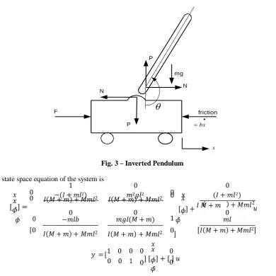
The pendulum moves vertically, the force 𝐹 is the control input of the cart that moves horizontally and the angular position of the pendulum 𝜃 and the horizontal position of the cart 𝑥 are the outputs. Also 𝑁 is the reaction force [14].

The motion in the cart is defined by

The motion in the pendulum is

𝑀𝑥 + 𝑏𝑥̇ + 𝑁 = 𝐹

(𝑀 + 𝑚)𝑥 + 𝑏𝑥̇ + 𝑚𝑙𝜃 𝑐𝑜𝑠𝜃 − 𝑚𝑙𝜃̇2_{𝑠𝑖𝑛𝜃 = 𝐹}

(𝐼 + 𝑚𝑙2_{)𝜃 + 𝑚𝑔𝑙𝑠𝑖𝑛𝜃 = −𝑚𝑙𝑥 𝑐𝑜𝑠𝜃}

(14)

(15)

(16) The system has to be linearized. The two linearized motion of the equations are

(𝐼 + 𝑚𝑙2_{)𝜙̈ − 𝑚𝑔𝑙𝜙̈ = 𝑚𝑙𝑥}

(𝑀 + 𝑚)𝑥 + 𝑏𝑥̇ − 𝑚𝑙𝜙̈ = 𝑢

The transfer function of the linearized system is

(17)

(18)

Φ(𝑠) 𝑈(𝑠)

𝑚𝑙 _𝑠2

= 𝑞

𝑠4 ₊𝑏(𝐼 + 𝑚𝑙2) _𝑠3 ₋( 𝑀 + 𝑚)𝑚𝑔𝑙 _𝑠2 ₋ 𝑏𝑚𝑔𝑙 _𝑠

where

𝑞 𝑞 𝑞

(19)

(9)

277

0

Fig. 3 – Inverted Pendulum

and the state space equation of the system is

1 0 0

𝑥 0

𝑥 0 −(𝐼 + 𝑚𝑙

2₎

𝐼(𝑀 + 𝑚) + 𝑀𝑚𝑙2 𝐼(𝑀 + 𝑚) + 𝑀𝑚𝑙𝑚2𝑔𝑙2 2 0 𝑥 0 𝑥̇ (𝐼 + 𝑚𝑙2)

( ) 2

[𝜙̈̇] = _{[𝜙̈] +}𝐼 𝑀 + 𝑚 + 𝑀𝑚𝑙 𝑢

0

𝜙̈ −𝑚𝑙𝑏 0 𝑚𝑔𝑙(𝑀 + 𝑚) 0 1 𝜙̈̇ 𝑚𝑙 0

0 _{𝐼(𝑀 + 𝑚) + 𝑀𝑚𝑙}₂ _{𝐼(𝑀 + 𝑚) + 𝑀𝑚𝑙}2 0]

𝑥

[𝐼(𝑀 + 𝑚) + 𝑀𝑚𝑙2_]

(20)

𝑦 = [1 0 0 0 𝑥 0 0 0 1 0] [𝜙̈] + [ ] 𝑢

𝜙̈̇

(21) Here the nonlinear plant is an Inverted Pendulum (IP) subject to parameter uncertainty without considering the cart movement for demonstration process. The proposed fuzzy controller is engaged for stabilizing the IP with IT2FLC. The dynamical equation of an IP is defined as follows:

(𝑎𝑚𝑝𝐿𝜃̇(𝑡)2 sin(2𝜃(𝑡))) 𝑔𝑠𝑖𝑛(𝜃(𝑡)) −

𝜃 (𝑡) = 4𝐿 2 − 𝑎 cos(𝜃(𝑡)) 𝑢(𝑡)

− 𝑎𝑚 𝐿𝑐𝑜𝑠2_(𝜃(𝑡))

3 𝑝

(22)

where 𝜃(𝑡) is the angular displacement of the pendulum, 𝑔 is the acceleration due to gravity, 𝑚𝑝 is the mass of the

pendulum, 𝑚𝑝 ∈ [𝑚 𝑝𝑚𝑖𝑛 , 𝑚𝑝𝑚𝑎𝑥 ] , 𝑎 =

1

(𝑚𝑝+𝑀𝑐) , 𝑀𝑝 ∈ [𝑀𝑐𝑚𝑖𝑛 , 𝑀𝑐𝑚𝑎��] , 𝑀𝑐 is the mass of the cart, 2𝐿 = 1𝑚 is the

length of the pendulum, 𝑢(𝑡) is the force applied to the cart and 𝑚𝑝, 𝑀𝑐 are regarded as the parameter uncertainties.

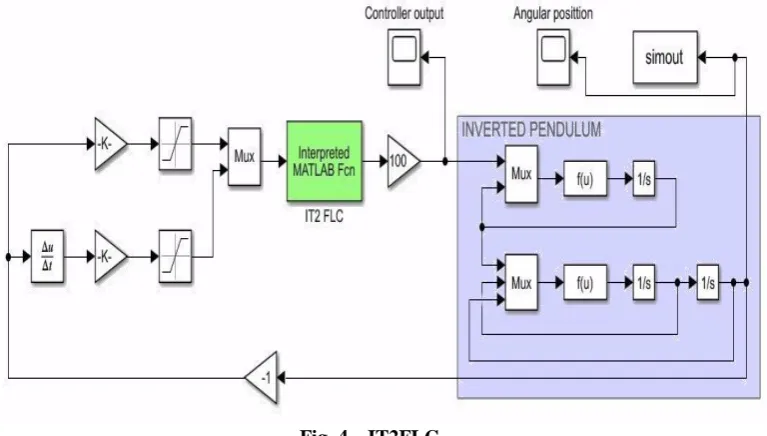
6.1 Interval Type-2 Fuzzy Logic Controller (IT2FLC)

P

mg

N N

F



P

friction

 bx

x

(10)

To fix the position of the input membership functions and uniformly distributed between -1 and +1. Limit these inputs to a minimum and maximum values using two saturation blocks Saturation 1 and saturation consecutively. The fuzzy controller is tuned by scaling gains. Control the spread of the input MFs by the input gains ‘Gain 1’ and ‘Gain 2’. To rescale the axes we can change gains. The MFs are uniformly spread out and contracted for the gains, which is less than 1 and greater than 1 respectively. The spread of the output MFs controlled by the output gain ‘Gain’ and the changes in it will lead to scale the vertical axis of the controller surface. If we increase the gains ‘Gain 1’ and ‘Gain 2’ then the proportional gain and the derivative gain in a PD controller will be increased respectively. If the proportional gain is increased then the system respond will be faster

Fig. 4 – IT2FLC

Controller Output

Speed

y

x Time

Fig. 5 - Chart for controller output

(11)

279

Angular Position

y Speed

x

Time

Fig. 6 - Chart for angular position

It shows its varying between the angular positions from 0 to 1.

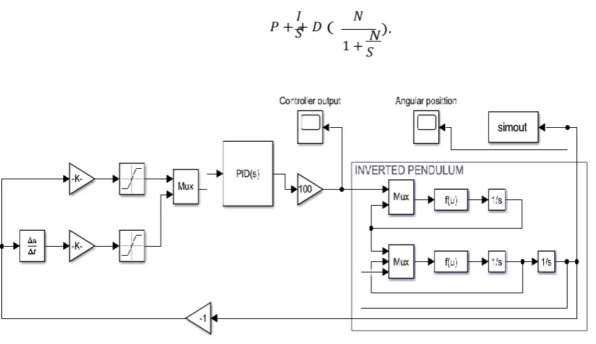
PID Control System

The transfer function is

𝐼

𝑃 + + 𝐷 ( _𝑆 𝑁 𝑁). 1 + 𝑆

Fig. 7 – PID Control System

(12)

Controller Output y

x Fig.8 – Chart for Controller Output

It shows that poor response. 𝑃 = 286.7, 𝐼 = 733.234, 𝐷 = 10081, Filter 𝑁 = 269.93 . The control output is not stationary and it’s getting decaying.

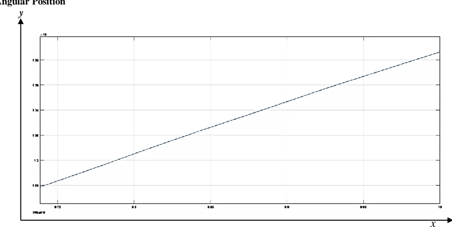
Angular Position

y

Fig. 9 – Chart for Angular Position

6.2 Comparison of Type-2 Fuzzy Controller and PID Controller

In process applications, PID controller is widely used but it has poor capability of controlling the system due to inadequate knowledge of the relation of input and output parameters, whereas Type-2 fuzzy logic controller has a very good capability in stability analysis with uncertainties in parameter. From this work, it is proved that IT2FLC deals with stability analysis better than PID controller.

(13)

281

7. Conclusion

The results reveal that Gaussian membership function gives the exact result with smoothness and T2FSs with interval MF, handles more uncertainties and less mathematical complexity than Type-1. Therefore GIT2MF is used and the mathematical properties of aggregation operator using IT2GWG operator are proved. These properties play an important role in control system for the characteristics like continuity, robustness and stability. In this research, IT2FLC is used to check the stability for an inverted pendulum and compared the result with PID controller that proved IT2FLC is better than PID controller for this system. For future research, it will be of interest to study other types of real world problems such as impulsive effects on optimal controller [20], directional change error evaluation [21], water consumptions expenditure [22], solid steel beam at elevated [23] in the framework of [24] and type-2 fuzzy controller.

References

[1] Lathamaheswari, M., Nagarajan, D., Kavikumar, J., & Chang Phang. (2018). A review on type-2 fuzzy controller on control system, Journal of Advanced Research in Dynamic & Control System, 10(11), 430-435. [2] Wu, D., & Tan, W.W. (2004). A type-2 fuzzy logic controller for the liquid-level process. Proceedings of IEEE

International Conference on Fuzzy Systems, 2(2), 953-958.

[3] Kobersi, I.S., & Finaev, V. I. (2013). Control of the heating system with fuzzy Logic. World Applied Sciences Journal, 23(11), 1441-1447.

[4] Rojas, I., Ortega, J., Pelayo, F.J., & Prieto, A. (1999). Statistical analysis of the main parameters in the fuzzy inference process, Fuzzy Sets and Systems, 102, 157-173.

[5] Bai. Y., & Wnag, D. (2006). Fundamentals of fuzzy logic control-fuzzy sets fuzzy rules and defuzzification. Advances Fuzzy Logic Technologies in Industrial Applications 17-36.

[6] Kayacan, E,. Kaynak, O,. Abiyer, R., & Jim, T. (2010). Design of an adaptive interval type-2 fuzzy logic controller for the position control of a servo system with an intelligent sensor. IEEE World Congress on Computational Intelligence 18-23.

[7] Tan, D.W.W.W. (2006). A simplified type-2 fuzzy logic controller for real time control. ISA Transactions, 45(4), 503-516.

[8] Dubois, D., & Prade, H. (2004). On the use of aggregation operations in information fusion processes. Fuzzy Sets and Systems, 142, 143-161.

[9] Klement, EP., Mesiar, R., & Pap, E. (2004). Triangular norms. Position paper III: continuous t-norms. Fuzzy Sets and Systems 145, 439-454.

[10] Volosencu, C. (2009). Stabilization of fuzzy control systems. WSEAS Transactions on Systems and Control, 3(10), 879-896.

[11] Franzoi, L., & Sgarro, A. (2017). Linguistic classification: T-norms, fuzzy distances and fuzzy distinguishabilities. Procedia Computer Science, 112, 1168-1177.

[12] Gaurav, A. (2012). Comparison between conventional PID and fuzzy logic controller for liquid flo control: Performance evaluation of fuzzy logic and PID controller by using MATLAB/Simulink. International Journal of Innovative Technology and Exploring Engineering, 1, 84-88.

[13] Lam, HK., & Seneviratne, LD. (2008). Stability analysis of interval type-2 fuzzy model-based control systems. IEEE Transactions on Systems, Man and Cybernetics-Part-B: Cybernetics, 38(3), 617-628.

[14] Ghosh, A., Krishnan, R., & Subudhi, B. (2012). Robust PID compensation of an inverted cart pendulum system. An experimental study. IET Control Theory & Applications, 6(8), 1145-1152.

[15] Zakwan, F.A.A., Krishnamoorthy, R.R., Ibrahim, A., & Ismail, R. (2018). A Finite Element (FE) simulation of naked solid steel beam at elevated temperature. International Journal of Integrated Engineering, 10(9), 96-102. [16] Khalib, S.N.B., Zakarya, I.A., & Izhar, T.N.T. (2018). Compositing of Garden Waste using Indigenous

Microorganisms (IMO) as Organic Additive. International Journal of Integrated Engineering, 10(9), 140-145. [17] Misri, Z., Wan Ibrahim, M.H., Halid, A.A., Awal, A.S.M., Shahidan, S., Faisal, S.K., Arshad, M.F., &

Ramadhansyah, P.J. (2018), Dynamic Mechanical Analysis of Waste Polyethylene Terephthalate Bottle. International Journal of Integrated Engineering, 10(9), 125-129.

[18] Ullah, K., Abdullah, A.H., Nagapan, S., Sohu, S., & Khan, M.S. (2018). Measures to Mitigate Causative Factors of Budget Overrun in Malaysian Building Projects. International Journal of Integrated Engineering, 10(9), 125- 129.

(14)

[20] Hamzah, N.S.B.A., Mamat, M.B., Kavikumar, J., Chong, L.S., & Ahmad, N.B. (2010). Impulsive differential equations by using the Euler method. Applied Mathematical Sciences, 4(65-68), 3219-3232.

[21] Nor, M.E., Rusiman, M.S., Mohamad, N.A.I., & Lee, M.H. (2017). Directional change error evaluation in time series forecasting. AIP Conference Proceedings, 1830(1), 080013.

[22] Razali, S.N.A.M., Rusiman, M.S., Zawawi, N.M., & Arbin, N. (2018). Forecasting of water consumptions expenditure using Holt-Winter’s and ARIMA. Journal of Physics: Conference Series, 995(1), 012041. [23] Hassan, S., Kumar, K., Raj, C.D., & Sridhar, K. (2014). Design and optimisation of pressure level using

metaheuristic approach. Applied Mechanics and Materials, 465-466, 401- 406.