Numerical Prediction of Temperature Distribution in Transient RTM Process

Numerical Prediction of Temperature Distribution in

Transient RTM Process

Shahnazari, Mohammad Reza*+

Mechanical Engineering Department, K.N.T University of Technology, Tehran, I.R. IRAN

Abbasi, Abbas

Mechanical Engineering Department, Amirkabir University of Technology, I.R. IRAN

Soltani, Majid

Mechanical Engineering Department, K.N.T University of Technology, Tehran, I.R. IRAN

ABSTRACT: Resin Transfer Molding (RTM) is a composite manufacturing process. A preformed fiber is placed in a closed mold and a viscous resin is injected into the mold. In this paper, a model is developed to predict the flow pattern, extent of reaction and temperature change during filling and curing in a thin rectangular mold. A numerical simulation is presented to predict the free surface and its interactions with heat transfer and cure for flow of a shear-thinning resin through the preformed fiber. To verify the model, the temperature profiles for preformed fiber have been calculated, and compared with the experimental results of other researchers. The results showed that, to optimize better quality of production of composite materials, while considering the effect of curing on temperature distribution during the process, the heat dispersion term should not be neglected.

KEY WORDS: Resin Transfers Molding (RTM), Porous media, Composites processing, Curing.

INTRODUCTION

Resin transfer molding (RTM) is becoming the most popular manufacturing process for composite materials because of its ability to manufacture complex shaped parts under low operation conditions.

In the RTM process, a liquid resin is injected into a mold where a fiber mat has been placed beforehand. As the result of heat activation, the filling is performed

before resin solidification. Since, the fiber orientation is perfectly controlled in this method, there are some advantageous of this process with respect to the conventional injection or compression molding of fiber suspension.

Heat transfer in a porous material depends on the molecular construction of medium. Therefore, during the * To whom correspondence should be addressed.

+ E-mail: mshahnazari@ nri.ac.ir

non-isothermal RTM process, conductive and convective heat transfers play important roles [1]. A convenient numerical modeling to analyze the heat transfer is based on the volumetric averaging of the field quantities.

The discrepancy between the microscopic thermal convection and the volumetric averaging is called the mechanical heat dispersion. The heat dispersion term was neglected by [2] in non-isothermal RTM process. Tucker and Dessenberger [3] showed that heat dispersion is important in typical RTM process by conducting a non-dimensional analysis. Dessenberger and Tucker [4] conducted some experiments by using random preform and compared the numerical results with and without dispersion term. Of course, they applied the local thermal equilibrium model in their study, which assumes that the fiber tows and resin system reach the same temperature instantaneously on contact. To simplify the analysis, the RTM process can be divided into mixing, filling and curing stages. A general overview of RTM modeling can be found in the review by Mal and Castro [5-6]. In the present paper, a model for the non-isothermal simulation of RTM is investigated. Also, the influence of the curing reaction on the filling is studied. The thermal behavior of the resin and the reinforcement is analyzed.

THEORY

To consider the mathematical model, the relevant dimensions according to experimental specimen were chosen. Fig. 1 shows a simple schematic of the process. The first average concept to be considered is porosity. It is defined as the local ratio of the volume to be filled by the liquid to the total volume.

V Vf f =

ε (1)

Fig.1: Schematics of the process

The average velocity vector < u f > is called the Darcy

velocity. This concept can directly provide the flow rate across any section. It differs from the intrinsic phase velocity < u f >f, which is defined as the average velocity

in the liquid phase only and provides the front flow velocity during filling. The relation links the Darcy and intrinsic phase velocities:

> =< >

< _f f _f

f u u

ε (2)

The assumptions which were used in this model are as follows:

- The flow is one-dimensional.(X only x-directinol component a Velocity is nonzero)

-

Local thermal equilibrium exists between the liquid and solid phases.

-

All the properties are constant.

-

There is no consolidation and the wetting and individual fibers play a negligible role as compared to the flow around the fiber bundles.

-

Heat transfer is convected in the X-direction and the conduction heat transfer is in the X and Y directions. The flow equation in the X-direction is the Darcy’s equation:

-

Newtonian fluid, that is, the viscosity is only an explicit function of the extent of reaction and temperature.

(

C,T

)

µ

µ = (3)

x p K u

f f xx

f _∂

∂ − =

µ (4)

It should be noted that other mathematical models which include inertia term like Forchheimer model, can be used. However, in this work, due to flow velocity ranges involved the Darcy’s equation has been applied. The temperature field plays a major role in the resin transfer molding and can strongly affect the flow through its influence on the fluid viscosity. Therefore, the effects of two phases must be taken into account in each equation, which will undoubtedly increase the accuracy of the results. The local thermal equilibrium assumption is completely valid for the process, for two reasons. Firstly, it is impossible to measure each phase temperature separately. Secondly, the characteristic time governing the heat transfer between the liquid and solid phases is small as compared with the process time scale.

Front Flow Resin In

Resin Out Resin In

As a result, a single temperature for solid and fluid must be considered: > =< > =< >

<Tf f Ts s T (5)

The subscripts f and s in the equation refer to the, liquid phase (resin) and solid phase (fiber mat), respectively. In order to get a unique energy equation, the contributions of the liquid and solid phases must be added. Hence, the resulting equation is as the follows:

( ) ( )

(

)

+

( )

< >∇< >=

∂ > < ∂

+ c . T

t T c

cp_s ερ p _f ρ p_f vf

ερ (6)

(

)

(

)

_   ∆ + > < ∇ ⋅ + ⋅

∇ k_e k_D T ε_fρ_f HF_c T f, C_f f

where cP denotes heat capacity, ke is average molecular

thermal diffusion tensor. and kD is the mechanical mixing

tensor. ∆H is the reaction heat and the function F(T,C) represents the curing kinetics. These two tensors can be explained as below:

∑

∫

=       ₊ = f , s

i i S i

e

inb dS

V 1 I

k ε (7)

(

)

₍

₎

∑

= −

∫

−< >

= _{i s,f i}

V i

i P

D u u b dV

V c k i ρ (8)

Where b shows the deviation vector between microscopic temperature and local equilibrium temperature which is:

> < ∇ ⋅ + >

=<T b T

Ti i (9)

The boundary conditions on the wall and at the inflow are the Dirichlet condition, and can be written as follows:

wall T T>=

< (10)

and front flow velocity is:

f f f

front u u

U ε > < = >

=< on the interface (11)

The species balance equation is written as follows:

(

< >⋅<∇ >

)

= + ∂ ∂ C u t C f f f ρ

ερ (12)

(

Dd⋅∇C

)

+εfρfFc T , C

⋅ ∇

where it is assumed that the molecular diffusion within the macro molecular medium is negligible, while mechanical dispersion is governed by the tensor Dd.

The energy equation for the local thermal equilibrinm model can be written as

( )

( )

{

}

( )

= ∂ ∂ + ∂ ∂ + x T u C t T C

Cp _sεs ρ p _fεf ρ p _{f x}

ρ (13)

( ) ( )

[

f

]

f f f c f f 2 2 yy 2 2

xx H F c , T

y T k

x T

k + ∆

        ∂ ∂ + ∂ ∂ ρ ε where hcx x Dxx exx

xx k k u c

k = + − (14)

Dyy eyy

yy k k

k = + (15)

( )

xi

f , s

i p i

hex c b

c =

∑

₌ ρ (16)

By definition, Pe=

( )

ρCp _f u dp /

(

2kf

)

, which dp is

the equivalent solid particle diameter . If a low peclet number is assumed,to the inclusion of kxx,chex can be

neglected because the energy equations in dimensioless for can be expressed as

( )

( )

[

]

( )

= ′ ∂ ′ ∂ ′ + ′ ∂ ′ ∂ + x T u x T x U C C C x c f p s f p s s p ρ ε ρ ε ρ (17)

( )

_{( )}

( )

C U T

T , C F H y T Uy C x k x T Ux C k f p f f f f c f f 2 2 c f p c yy 2 c f p xx ∆     ∆ +         ′ ∂ ′ ∂ + ′ ∂ ′ ∂ ρ ρ ε ρ ρ low wall low T T T T T inf inf − − =

′ (18)

D x

x u /u

u′ = (19)

c x

x

x′= (20)

h y

y= (21)

c t

t

t′= (22)

Here h is the mold half thickness,uD is the Darcy

velocity and the charactristic leugth xc can be obtained .

For a thin mold cavity and without reaction heat source, the volume – averaged energy equation for the quasi-steady state simplifies to

( )

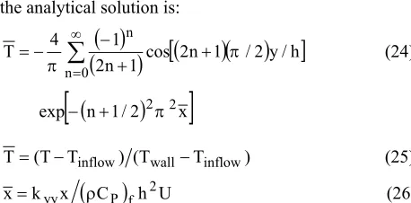
2

the analytical solution is:

( )

(

)

[

(

)(

)

]

∑

∞ = + + − − = 0 n n h / y 2 / 1 n 2 1 n 2 1 4 T π

π cos (24)

exp

[

−

(

n+1/2

)

2π2x

]

) T T ( ) T T (

T= − inflow wall− inflow (25)

(

C

)

h U

x k

x= _yy ρ _{P f} 2 (26)

This allows one to solve for xc one can now compare the

magnitude of conduction effects in dimensionless equation to formulate a criterion for neglecting x-direction conduction as

1 h

x k

k _c 2

xx yy >>       (27)

For Pe>>1, By xc calculation this can be shown ,that

the above criterion is valid [7].

For exampel, with Pe=1.4,xc=0.52, 2704 h

x_c 2

=      

and the inequality 1

h x k

k _c 2

xx yy _>>              

holds, because

k

has the same mgnitude of k.

Therefore, the energy and species balance equations can be written as the follows:

(

)

( )

= ∂ ∂ > < + ∂ > < ∂ + x T u C t T ) C ( ) C

(ερ p s ερ p f ρ p _f x (28)

( )

H

y T

K ₂ f f

2

yy + ∆

∂ > < ∂

ρ

ε Fc

[

T, C

]

and >= ∇ < ⋅ > < + ∂ ∂ C v y C f f

fε ρ

ρ (29)

[

T, C

]

F y

C

D ₂ f f c

2

d +ε ρ

∂ > < ∂

The kinetic mechanism is more complex than simple second order [6]. However for process modeling what, had to be used as the only phenomenological reaction is:

2 o

c(T,C) A ( _RTE )C

F = exp− (30)

        −         = C C C RT E A g g µ µ

µ exp (31)

T B A

Cg = c + c (32)

NUMERICAL METHOD

A non-uniform grid,together with higher - order finite difference approximations that use nearest and next nearest neighbors, have be used in order to predction of free surface position the MAC method was modified by including irregular grid mesh and a trial and error scheme. The highly nonlinear character of equations suggests applying a decoupled iterative solution strategy for this purpose, the simulation comprises a set of modules devoted to calculate the pressure, velocity, temperature and conversion degree fields at each time step separately.

The calculation begins at the mold entrance at each time step and proceeds upstream. The program switches from main flow to flow front. The global algorithm manages the interaction between the different modules. A simple iterative strategy was selected. From the knowledge of all fields at time tnand an estimate of

these fields at time tn+1, a new estimate of these fields is

obtained at time tn+1. The values of velocity components

over the constant displacement curvature of each cell can be related to the velocity components of each mesh using Taylor’s series. A trial and error method was applied to increase the accuracy of the results, as follows:

(

u u

)

t

xnew = n_k 1− n_k ∆

∆ + (33)

To solve, energy and species balance equations, an implicit finite difference method has been applied. All

x T ∂ > ∂ < and x C ∂ > < ∂

terms in the equations, the

boundary conditions in form of upwind and second order terms in equation are discretized by central difference. The successive temporary meshes are generated during the filling to evaluate the pressure and temperature profiles. Therefore, the calculations are decoupled.

NUMERICAL RESULTS

Thermal Couductivity And Thermal Dispersion

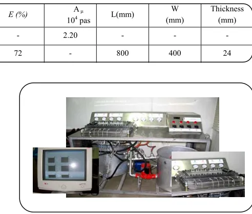
The material data used in the simulations are given in table 1 and the reological and kinetic parameters are given in table 2. The composite thermal conductivity is a function of the conductivity of the phases through the Chang’s model [8].

Table 1: material parameters for the resin preformed fiber and system

ρ

kg / m3

CP

J /kgK

K

W / (mK) E (%)

Aµ

104 _pas L(mm)

W (mm)

Thickness (mm)

Resin 1202 2800 0.276 - 2.20 - - -

Preformed Fiber 2560 670 0.417 72 - 800 400 24

Table 2: Rheological and kinetic parameters

A0 (m3 / mols) 36000

E (Kg / mol) 57.8

∆H (kg / mol) 83

Av 1.5

Bv 1

Ac 0.44

Bc 0.0045

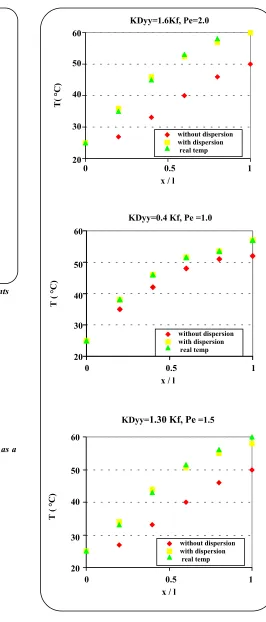
Once experimental system was can structed for mold temperature instrumentation. Experiments were performed using a non-curing fluid to avoid complications caused by exothermic reactions that actual resin systems undergo. The fluid used was a mixture of 2/3 Glycerine and 1/3 Ethylene Glycol. The experimental equipment is shown in Fig. 2. Water was circulated through the small ducts inside th mold walls in order to hold the wall temperatures .

Eighteen thermocouples (0.9 mm diameter, error in 0.3 percent) were arranged perpendicular to the flow direction. To model the mechanical dispersion term the conservation equations are as follows:

u b ) c (

K_dyy = ερ _{p f yy} (35)

yy f f

dyy ub

D =ε ρ (36) in order to determine the thermel disperssion, the energy equation was solved for non-curing system, for different kyy values and compared by this experiment results.

RESULTS AND DISCUSSION

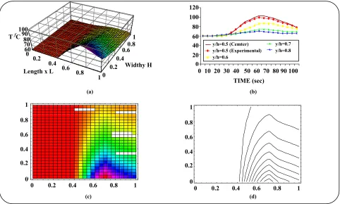
The front flow position at different pressure gradients have been shown in Fig. 3. As is seen, the process time gradually decreases as the pressure gradient increases. Using the Chang`s model for non-curing system, Fig. 4 shows the quasi steady temperature distribution without consideration of the curing for different value of thermal disspersion in comparison with experrimental data. In summar, from the set of numenial analysis and experiments, the significance of heat dispersion

Fig. 2: A photograph of the experimental system

(kyy-ke=kDyy) is verfied and validated in RTM.

Fig. 5 shows the values of kDyy used to match the

experimental data is a function of Peclet number, Also, Fig. 6 compares the temperature distribution with that of Hsiao et. al. [9]. The effect of curing on the temperature distribution in different position of the medium is shown in Fig. 7. These results show that during curing, the temperature rises up to a maximum value and then decreases due to the heat conduction to the mold walls. Also, for the thicker Fig. 8 shows the corresponding results for the thicker mold. In this case, the maximum temperature value is smaller, but there is still a large temperature difference between the center and that of the wall proximity. The reason is the difference in properties at the center and at the wall.

CONCLUSIONS

(a)

(b)

Fig. 3: Flow front position at different pressure gradients

Fig.5: The kdyy value for matching the experimental data as a

function of the Pe Number

Fig.6: The non-curing transient RTM process temperature profiles, comparison of theoretical and experimental data.

Fig. 4: Quasi steady state temperature profile for non- curing RTM process distribution

0 0.5 1 1.5 2 2.5

2 3 4 5 6

Pe

Kdyy

2 3 4 5 6 Pe

2.5

2

1.5

1

0.5

0

Kdyy

0 10 20 30 40 50 60 70

2 22 42 62 82 102 122 142 162 188 208

x/l=.2 x/l=.4 x/l=.6 x/l=.8 x/l=.9 x/l=.6[9] x/l=.4 Exp. x/l=.8 Exp. x/l=0.8[9]

2 42 82 122 162 208 Time (sec)

70 60 50 40 30 20 10 0

Temp x/l=.4

x/l=.8 x/l=0.6 [9] x/l=.8 Exp.

x/l

0

0.2

0.4

0.6

0.8

1

1.2

0

25

50

75

100

Grad P=37.5KPa Grad P=50KPa Grad P=100KPa

1.2

1 0.8

0.6

0.4

0.2 0

0 25 50 75 100 Time (sec)

Grad P = 37.5 KPa Grad P = 50 KPa Grad P = 100 KPa

T( °C)

20 30 40 50 60

0 0.5 1

60

50

40

30

20

0 0.5 1 x / l

KDyy=1.6Kf, Pe=2.0

without dispersion with dispersion real temp

20 30 40 50 60

0 0.5 1

0 0.5 1 x / l

KDyy=0.4 Kf, Pe =1.0 60

50

40

30

20

without dispersion with dispersion real temp

T ( °C)

20 30 40 50 60

00 0.5 1 0.5 1 x / l

60

50

40

30

20

KDyy=1.30 Kf, Pe =1.5

without dispersion with dispersion real temp

T ( °C)

(a) (b)

(c) (d)

Fig.7: RTM’s temperature distribution when curing is considered (H=2 mm)

(a) (b)

(c) (d)

Fig. 8: RTM’s temperature distribution when curing is considerated (H=4 mm)

TEMP

0 20 40 60 80 100 120

0 _{10 20 30 40 50 60 70 80}

TIME ( sec. )

TEM

P

y/h=0.5( Center ) y/h=0.5(Experimental)

y/h=0.6 y/h=0.7

y/h=0.8

120 100 80 60 40 20 0

0 10 20 30 40 50 60 70 80 TIME (sec.)

y/h=0.5 (Cemter) y/h=0.6 y/h=0.8

y/h=0.5 (Experimental) y/h=0.7

0 0. 2

0. 4 0. 6

0. 8 1

Le ng thx L

0 0. 2

0. 4 0. 6

0. 8 1

Wi dt hy H

60 80 10 0 12 0

T Cƒ

0 0. 2

0. 4 0. 6

0. 8 1

Le ng thx L

1 0.8 0.6 0.4 0.2 1 0 0.8 0.6 0.4 0.2 0 60 80 100 120 T f_C

Lengthx L

widthy H

0 0.2 0.4 0.6 0.8 1

0 0.2 0.4 0.6 0.8 1

1

0.8

0.6

0.4

0.2

0

0 0.2 0.4 0.6 0.8 1

0 0.2 0.4 0.6 0.8 1

0 0.2 0.4 0.6 0.8 1

1

0.8

0.6

0.4

0.2

0

0 0.2 0.4 0.6 0.8 1

0 0.2 0.4 0.6 0.8 1

0 0.2 0.4 0.6 0.8 1

0 0.2 0.4 0.6 0.8 1 1

0.8

0.6

0.4

0.2

0

0 0.2 0.4 0.6 0.8 1 0

0.2 0.4 0.6 0.8 1

0 0.2 0.4 0.6 0.8 1 1

0.8

0.6

0.4

0.2

0

0 0.2

0.4 0.6

0.8

10

0.2 0.4

0.6 0.8

1

60 70 80 90 100

T Cƒ

0 0.2

0.4 0.6

0.8 1

1 0.8 0.6 0.4 0.2 0 1 0.8 0.6 0.4 0.2 0 60 70 80 90 100 T f_C

Widthy H Length x L

0 20 40 60 80 100 120

0 10 20 30 40 50 60 70 80 90 100

TIME ( sec. ) TE

M P

0 10 20 30 40 50 60 70 80 90 100 TIME (sec)

120 100 80 60 40 20 0

y/h=0.5 (Cemter) y/h=0.5 (Experimental) y/h=0.6

Nomenclature

Ao Constant in the kinetic equation (30)

Ac Constant in the max conversion equation (eq.32)

Aµ Constant in the viscosity equation (31)

Av Constant in the viscosity equation (31)

b Vector function for transforms the average temperature gradient into the pointwise temperature deviation Bc Constant in the max conversion equation (32)

Bv Constant in the viscosity equation (31)

Cp Specific heat

C Conversion of chemical species Cg Max conversion

Chex

∑

_i=s,f

( )

ρcp _i bxi

D Mess difusivity E Activation energy in kinetic equation (eq.30) EM Activation energy in viscosity equation (eq.31)

Fc Reaction Function

H Mold half height I Unit tensor k Thermal conductivity k Permeability tensor

π Unit outward normal vector P Pressure t Time T Temperature Tinflow Input temperature of fluid

U Velocity component V Velocity vector x,y,z Coordinats

ε Volume fractions

µ Resin viscosity

ρ Density

∆H Heat of reaction

<> Volume average

<>f_,<>s _{Intrinsic phase averages over the fluid}

and solid phase

Subscripts

f Fluid (resin) s Solid (fiber) i (solid and fluid)

ω Wall e Eflective D Disperssion C Charactristic

Received : 24th _{May 2003 ; Accepted : 27}th _{November 2003}

REFERENCES

[1] Bruscke, M.V. and Advani, S.G. “A numerical Approach to model, Non-isothermal, viscous flow with free surface through fibrous media” Int. J. Numer. Methods Fluids,19, P. 575 (1994).

[2] Liu, B. and Advani, S.G. “Operator splitting scheme for 3-D flow approximation” Computational Mechanics, J., 38, P. 74 (1995).

[3] C. Tucker. C.L. and Dessenberger. R.B., “Governing equations for flow and heat transfer in stationary fiber beds” In flow and Rheology in Polymer Composites Manufacturing, chap.8, edited by, S.G. Advani, Elsevier, Amsterdam, p. 257-323 (1994). [4] Dessenberger, R. D. and Tucker, C. L., “ Thermal

dispersion in resin transfer molding”, polymer composites,16 (6) 495 (1995).

[5] Mal, O., Couniut, A. and Depert, F., “ Non-isothermal simulation of the resin transfer molding process”, Composites part A, 29,p. 180 (1998). [6] Castro. J. and Macosko. C., “Studies of mold filling

and curing in the reaction injection molding process”, AIChe., J. 2000, 28, 250 (1982).

[7] Shahnazari, M.R., Abbassi, A., Transient Numerical Simulation of Non-Isothermal process of RTM, proccedings of 4th _{ASME/JSME joint Fluid}

Engineeing, FEDSM`03, july 6-11 Hawaii, USA, (2003).

[8] Kaviany, M., Principle of Heat Transfer in Porous Media, Springer-Verlag, New York, (1991).